This page was generated from
docs/examples/mineralML_synthetic_data.ipynb.
Interactive online version:
![]() .
.
[1]:
""" Created on November 13, 2023 // @author: Sarah Shi """

import os
import numpy as np
import pandas as pd

import mineralML as mm

import matplotlib.pyplot as plt
%matplotlib inline
%config InlineBackend.figure_format = 'png'
Synthetic Mineral Generator
This notebook shows how the synthetic mineral generator in mineralML works, with an example CSV for groundtruthing: training_hundred.csv. This is a three step process:
Load and prepare data for analysis.
Define endmembers and generator settings (e.g.,
oxygen_basis, mixing distribution/parameters, minor elements, noise scales).Generate synthetic compositions and evaluate them (convert to oxide wt% and cations; optionally use
compare_distributionsto compare against the natural dataset).
We loaded in the mineralML Python package as mm. mineralML has trained machine learning models for classifying minerals. This implementation aims to get your electron microprobe or quantitative EDS compositions classified and processed. We remove some degrees of freedom to simplify the process as much as possible. The minerals considered for this study include: Amphibole, Apatite, Biotite, Calcite, Chlorite, Epidote, Feldspar (KFeldspar and Plagioclase), Garnet, Glass, Kalsilite,
Leucite, Melilite, Muscovite, Nepheline, Olivine, Pyroxene (Clinopyroxene and Orthopyroxene), Quartz, Rhombohedral_Oxides (Hematite-Ilmenite), Rutile, Serpentine, Spinels (Magnetite-Spinel), Titanite, Tourmaline, and Zircon.
One CSV file containing your electron microprobe analyses in oxide weight percentages is necessary. Find an example here. The necessary oxides are \(SiO_2\), \(TiO_2\), \(Al_2O_3\), \(FeO_t\), \(MnO\), \(MgO\), \(CaO\), \(Na_2O\), \(K_2O\), \(Cr_2O_3\), and \(P_2O_5\). For the oxides not analyzed for specific minerals, the preprocessing will fill in the nan values as 0.
Load and prepare data for groundtruthing
[2]:
# Read in your dataframe of mineral data, called training_hundred.csv.
# Prepare the dataframe by removing rows with too many NaNs, and filling in zeros.

df_load = mm.load_df('TabularData/synth_groundtruth.csv')
[3]:
# Examine the prepared dataframe

display(df_load.head())
| Sample Name | SiO2 | TiO2 | Al2O3 | FeOt | MnO | MgO | CaO | Na2O | K2O | P2O5 | Cr2O3 | Mineral | |
|---|---|---|---|---|---|---|---|---|---|---|---|---|---|
| 43110 | CN_C_Ol1 | 39.846040 | 0.000020 | 0.019150 | 17.398750 | 0.243865 | 43.126690 | 0.219630 | 0.014950 | 0.007775 | 0.013685 | NaN | Olivine |
| 43111 | CN_C_Ol1' | 39.787840 | 0.010270 | 0.026165 | 17.446295 | 0.324905 | 43.227635 | 0.188190 | 0.015305 | 0.006115 | 0.017815 | NaN | Olivine |
| 43112 | CN_C_Ol2 | 38.896455 | 0.014615 | 0.005655 | 21.791545 | 0.349310 | 39.472920 | 0.204635 | 0.004635 | 0.006005 | 0.013985 | NaN | Olivine |
| 43113 | CN_C_Ol3 | 39.451170 | 0.000020 | 0.028775 | 19.528820 | 0.298085 | 41.429130 | 0.231755 | 0.000010 | 0.001825 | 0.019815 | NaN | Olivine |
| 43114 | CN_C_Ol3_MI2 | 39.680195 | 0.006940 | 0.019405 | 18.502340 | 0.303840 | 42.207405 | 0.226190 | 0.018970 | 0.000010 | 0.000020 | NaN | Olivine |
Olivine
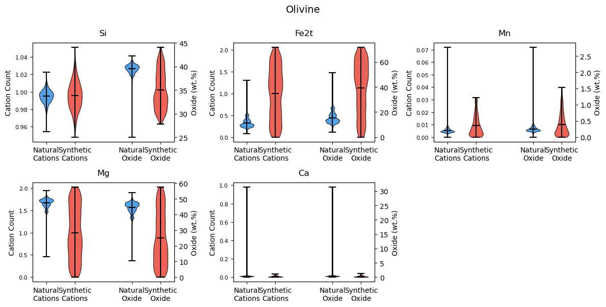
Let’s apply the generator to olivine as a simple binary solid solution between forsterite (Mg₂SiO₄) and fayalite (Fe₂SiO₄). We understand olivine systematics quite well, so we can test this before applying this to a more complex system. We will keep everything on a 4-oxygen basis, add small amounts of Ca and Mn as minors, and then check that the synthetic cloud matches the natural data. The steps are as follows:
Define endmembers (4 oxygen basis). Use cation counts per formula unit; iron as total cations (
Fe2t) so the framework can convert toFeOtdownstream.Specify minor elements (optional but realistic).
Instantiate the generator with
mm.SolidSolutionGenerator.Generate synthetic compositions.
Compute sites/derived components.
Compare synthetic vs natural distributions with
compare_distributions.Plot paired violin distributions for cations (and matching oxides if present). Report KS statistics (
ks_stat,p_value) plus means/stds. Lowerks_stat/ higherp_valuemeans a better match.
Gotchas:
Keep iron conventions straight:
Fe2t(cations) aligns withFeOt(oxide). Don’t mix FeO/Fe₂O₃ with FeOt in the same row.
[4]:
# Pull natural data
df_ol_natural = df_load[df_load["Mineral"]=="Olivine"]
ol_calc_natural = mm.OlivineCalculator(df_ol_natural)
ol_comp_natural = ol_calc_natural.calculate_components()
# Define endmembers
ol_endmembers = {
# Forsterite: Mg₂SiO₄
'Fo': {'Mg': 2, 'Si': 1, 'O': 4},
# Fayalite: Fe₂SiO₄
'Fa': {'Fe2t': 2, 'Si': 1, 'O': 4}
}
# Specify minor elements
ol_minors = {
'Ca': {'distribution': 'exponential', 'scale': 0.01, 'max_fraction': 0.01},
'Mn': {'distribution': 'exponential', 'scale': 0.01, 'max_fraction': 0.01}
}
# Instantiate generator
ol_gen = mm.SolidSolutionGenerator(
endmembers=ol_endmembers,
oxygen_basis=4,
element_noise_scale=0.025,
min_site_fraction=0.2,
minor_elements=ol_minors,
mixing_dist='beta',
mixing_params={'a': 1, 'b': 1}
)
# Generate samples, use the olivine calculator to calculate site allocations, etc.
df_ol = ol_gen.generate(1000)
ol_calc_synth = mm.OlivineCalculator(df_ol)
ol_comp_synth = ol_calc_synth.calculate_components()
display(ol_comp_synth)
# Calculate and compare the distributions of the output data
stats_ol = ol_gen.compare_distributions(base_df=ol_comp_natural, synth_df=ol_comp_synth, suptitle="Olivine")
display(stats_ol)
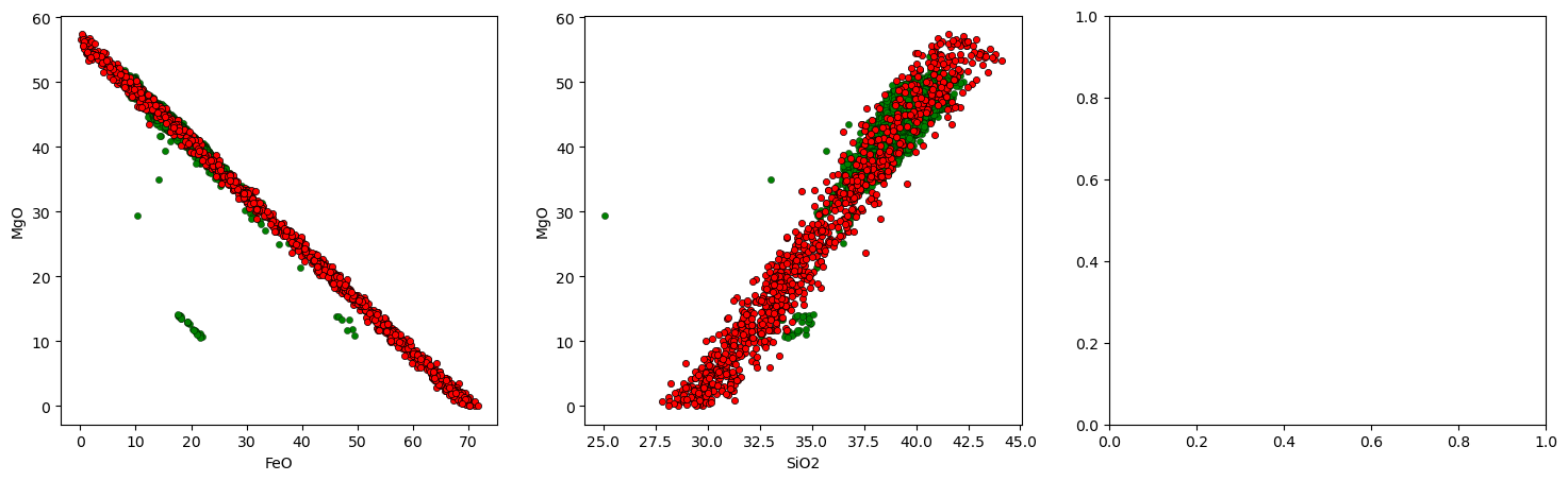
# Scatter‐plot comparing base vs. synthetic oxide proportions
fig, ax = plt.subplots(1, 3, figsize=(18, 5))
ax[0].scatter(ol_comp_natural["FeOt"], ol_comp_natural["MgO"], s=20, c="g", lw=0.25, ec='k')
ax[0].scatter(ol_comp_synth["FeOt"], ol_comp_synth["MgO"], s=20, c="r", lw=0.5, ec='k')
ax[0].set_xlabel("FeO")
ax[0].set_ylabel("MgO")
ax[1].scatter(ol_comp_natural["SiO2"], ol_comp_natural["MgO"], s=20, c="g", lw=0.25, ec='k')
ax[1].scatter(ol_comp_synth["SiO2"], ol_comp_synth["MgO"], s=20, c="r", lw=0.5, ec='k')
ax[1].set_xlabel("SiO2")
ax[1].set_ylabel("MgO")
ax[2].scatter(ol_comp_natural["XFo"], ol_comp_natural["M_site_expanded"], s=20, c="g", lw=0.25, ec='k', label="Natural")
ax[2].scatter(ol_comp_synth["XFo"], ol_comp_synth["M_site_expanded"], s=20, c="r", lw=0.25, ec='k', label="Synthetic")
ax[2].set_xlabel("XFo (Mg/(Mg+Fe))")
ax[2].set_ylabel("M-site Expanded")
ax[2].legend()
plt.tight_layout()
Charge mismatch: 9.01 vs 8
Charge mismatch: 9.39 vs 8
Charge mismatch: 8.87 vs 8
Charge mismatch: 7.12 vs 8
Charge mismatch: 8.97 vs 8
Charge mismatch: 7.19 vs 8
Charge mismatch: 8.82 vs 8
Charge mismatch: 8.92 vs 8
Charge mismatch: 9.43 vs 8
Charge mismatch: 7.07 vs 8
Charge mismatch: 8.95 vs 8
Charge mismatch: 7.18 vs 8
Charge mismatch: 9.01 vs 8
Charge mismatch: 7.08 vs 8
Charge mismatch: 7.06 vs 8
Charge mismatch: 8.85 vs 8
Charge mismatch: 9.11 vs 8
Charge mismatch: 8.85 vs 8
Charge mismatch: 8.83 vs 8
Charge mismatch: 9.11 vs 8
Charge mismatch: 7.01 vs 8
Charge mismatch: 6.98 vs 8
Charge mismatch: 9.05 vs 8
Charge mismatch: 8.86 vs 8
Charge mismatch: 8.81 vs 8
Charge mismatch: 7.14 vs 8
Charge mismatch: 7.15 vs 8
Charge mismatch: 8.82 vs 8
Charge mismatch: 8.81 vs 8
Charge mismatch: 7.00 vs 8
Charge mismatch: 7.15 vs 8
Charge mismatch: 8.90 vs 8
Charge mismatch: 9.21 vs 8
Charge mismatch: 7.18 vs 8
Charge mismatch: 6.95 vs 8
Charge mismatch: 7.05 vs 8
Charge mismatch: 7.08 vs 8
Charge mismatch: 7.16 vs 8
Charge mismatch: 7.09 vs 8
Charge mismatch: 7.13 vs 8
Charge mismatch: 8.81 vs 8
Charge mismatch: 7.20 vs 8
Charge mismatch: 9.19 vs 8
Charge mismatch: 7.16 vs 8
Charge mismatch: 7.12 vs 8
Charge mismatch: 9.54 vs 8
Charge mismatch: 6.79 vs 8
Charge mismatch: 8.95 vs 8
Charge mismatch: 9.07 vs 8
Charge mismatch: 9.29 vs 8
Charge mismatch: 8.86 vs 8
Charge mismatch: 8.81 vs 8
Charge mismatch: 8.87 vs 8
Charge mismatch: 8.84 vs 8
Charge mismatch: 8.88 vs 8
Charge mismatch: 8.97 vs 8
Charge mismatch: 9.77 vs 8
| Sample | SiO2 | FeOt | MnO | MgO | CaO | SiO2_mols | FeOt_mols | MnO_mols | MgO_mols | ... | Predict_Mineral | Prediction_Score | Prediction_Score_Sigma | Second_Predict_Mineral | Second_Prediction_Score | Cation_Sum | M_site | T_site | M_site_expanded | Fo | |
|---|---|---|---|---|---|---|---|---|---|---|---|---|---|---|---|---|---|---|---|---|---|
| 0 | NaN | 34.622234 | 41.032973 | 0.541935 | 23.626166 | 0.176691 | 0.576269 | 0.571140 | 0.007640 | 0.586193 | ... | NaN | NaN | NaN | NaN | NaN | 3.006716 | 1.994833 | 0.993284 | 2.013432 | 0.506503 |
| 1 | NaN | 36.787297 | 30.920356 | 0.630162 | 31.473580 | 0.188606 | 0.612305 | 0.430382 | 0.008883 | 0.780897 | ... | NaN | NaN | NaN | NaN | NaN | 2.999557 | 1.979104 | 1.000443 | 1.999114 | 0.644688 |
| 2 | NaN | 29.930481 | 65.841998 | 0.553641 | 3.647932 | 0.025948 | 0.498177 | 0.916458 | 0.007805 | 0.090510 | ... | NaN | NaN | NaN | NaN | NaN | 3.009386 | 2.002332 | 0.990614 | 2.018772 | 0.089883 |
| 3 | NaN | 38.550577 | 18.016443 | 0.170479 | 43.039413 | 0.223088 | 0.641654 | 0.250772 | 0.002403 | 1.067859 | ... | NaN | NaN | NaN | NaN | NaN | 3.015989 | 2.022191 | 0.984011 | 2.031978 | 0.809824 |
| 4 | NaN | 37.177048 | 32.068149 | 0.758269 | 29.973814 | 0.022720 | 0.618792 | 0.446358 | 0.010689 | 0.743686 | ... | NaN | NaN | NaN | NaN | NaN | 2.985055 | 1.951913 | 1.014945 | 1.970110 | 0.624923 |
| ... | ... | ... | ... | ... | ... | ... | ... | ... | ... | ... | ... | ... | ... | ... | ... | ... | ... | ... | ... | ... | ... |
| 995 | NaN | 36.612935 | 27.910138 | 0.174822 | 34.608587 | 0.693518 | 0.609403 | 0.388483 | 0.002464 | 0.858680 | ... | NaN | NaN | NaN | NaN | NaN | 3.017409 | 2.010904 | 0.982591 | 2.034818 | 0.688507 |
| 996 | NaN | 43.656266 | 1.857720 | 0.477573 | 53.888113 | 0.120327 | 0.726636 | 0.025858 | 0.006732 | 1.337028 | ... | NaN | NaN | NaN | NaN | NaN | 2.971148 | 1.929726 | 1.028852 | 1.942296 | 0.981027 |
| 997 | NaN | 36.625604 | 27.030119 | 0.793513 | 34.874823 | 0.675940 | 0.609614 | 0.376233 | 0.011186 | 0.865286 | ... | NaN | NaN | NaN | NaN | NaN | 3.018330 | 1.999236 | 0.981670 | 2.036660 | 0.696957 |
| 998 | NaN | 40.456203 | 8.932501 | 0.083621 | 50.038740 | 0.488935 | 0.673372 | 0.124332 | 0.001179 | 1.241521 | ... | NaN | NaN | NaN | NaN | NaN | 3.010654 | 2.006766 | 0.989346 | 2.021308 | 0.908971 |
| 999 | NaN | 31.582903 | 55.343212 | 0.243916 | 12.732789 | 0.097179 | 0.525681 | 0.770325 | 0.003438 | 0.315916 | ... | NaN | NaN | NaN | NaN | NaN | 3.018691 | 2.027728 | 0.981309 | 2.037382 | 0.290834 |
1000 rows × 33 columns
(<Figure size 1200x600 with 11 Axes>,
                ks_stat        p_value  mean_base  mean_synth  std_base  \
 cation
 Si_cat_4ox    0.213778   7.300022e-39   0.994964    0.995663  0.007191
 Fe2t_cat_4ox  0.703333   0.000000e+00   0.327584    0.998053  0.094729
 Mn_cat_4ox    0.380164  7.802087e-125   0.005196    0.009274  0.002395
 Mg_cat_4ox    0.703054   0.000000e+00   1.664797    0.992028  0.104283
 Ca_cat_4ox    0.348305  2.934413e-104   0.009132    0.009319  0.032880

               std_synth
 cation
 Si_cat_4ox     0.016431
 Fe2t_cat_4ox   0.589282
 Mn_cat_4ox     0.008350
 Mg_cat_4ox     0.587416
 Ca_cat_4ox     0.008193  )
---------------------------------------------------------------------------
KeyError                                  Traceback (most recent call last)
File ~/checkouts/readthedocs.org/user_builds/mineralml/conda/stable/lib/python3.9/site-packages/pandas/core/indexes/base.py:3812, in Index.get_loc(self, key)
   3811 try:
-> 3812     return self._engine.get_loc(casted_key)
   3813 except KeyError as err:

File pandas/_libs/index.pyx:167, in pandas._libs.index.IndexEngine.get_loc()

File pandas/_libs/index.pyx:196, in pandas._libs.index.IndexEngine.get_loc()

File pandas/_libs/hashtable_class_helper.pxi:7088, in pandas._libs.hashtable.PyObjectHashTable.get_item()

File pandas/_libs/hashtable_class_helper.pxi:7096, in pandas._libs.hashtable.PyObjectHashTable.get_item()

KeyError: 'XFo'

The above exception was the direct cause of the following exception:

KeyError                                  Traceback (most recent call last)
Cell In[4], line 53
     50 ax[1].set_xlabel("SiO2")
     51 ax[1].set_ylabel("MgO")
---> 53 ax[2].scatter(ol_comp_natural["XFo"], ol_comp_natural["M_site_expanded"], s=20, c="g", lw=0.25, ec='k', label="Natural")
     54 ax[2].scatter(ol_comp_synth["XFo"], ol_comp_synth["M_site_expanded"], s=20, c="r", lw=0.25, ec='k', label="Synthetic")
     55 ax[2].set_xlabel("XFo (Mg/(Mg+Fe))")

File ~/checkouts/readthedocs.org/user_builds/mineralml/conda/stable/lib/python3.9/site-packages/pandas/core/frame.py:4107, in DataFrame.__getitem__(self, key)
   4105 if self.columns.nlevels > 1:
   4106     return self._getitem_multilevel(key)
-> 4107 indexer = self.columns.get_loc(key)
   4108 if is_integer(indexer):
   4109     indexer = [indexer]

File ~/checkouts/readthedocs.org/user_builds/mineralml/conda/stable/lib/python3.9/site-packages/pandas/core/indexes/base.py:3819, in Index.get_loc(self, key)
   3814     if isinstance(casted_key, slice) or (
   3815         isinstance(casted_key, abc.Iterable)
   3816         and any(isinstance(x, slice) for x in casted_key)
   3817     ):
   3818         raise InvalidIndexError(key)
-> 3819     raise KeyError(key) from err
   3820 except TypeError:
   3821     # If we have a listlike key, _check_indexing_error will raise
   3822     #  InvalidIndexError. Otherwise we fall through and re-raise
   3823     #  the TypeError.
   3824     self._check_indexing_error(key)

KeyError: 'XFo'
Feldspar
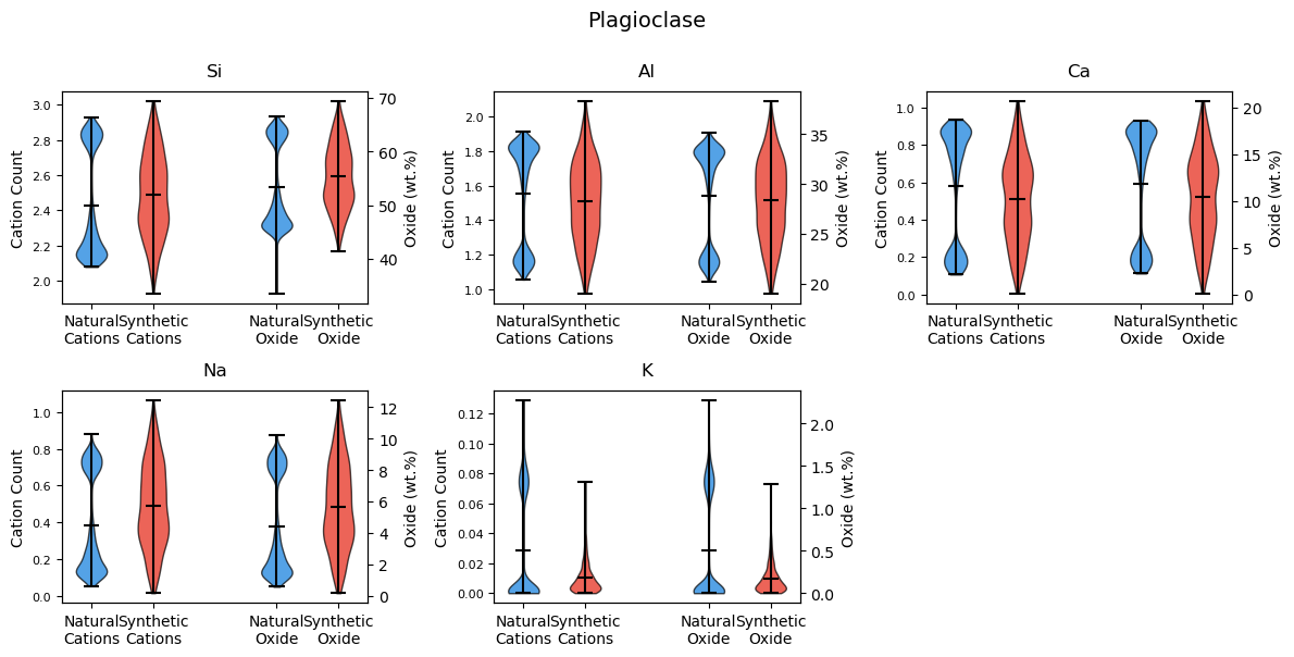
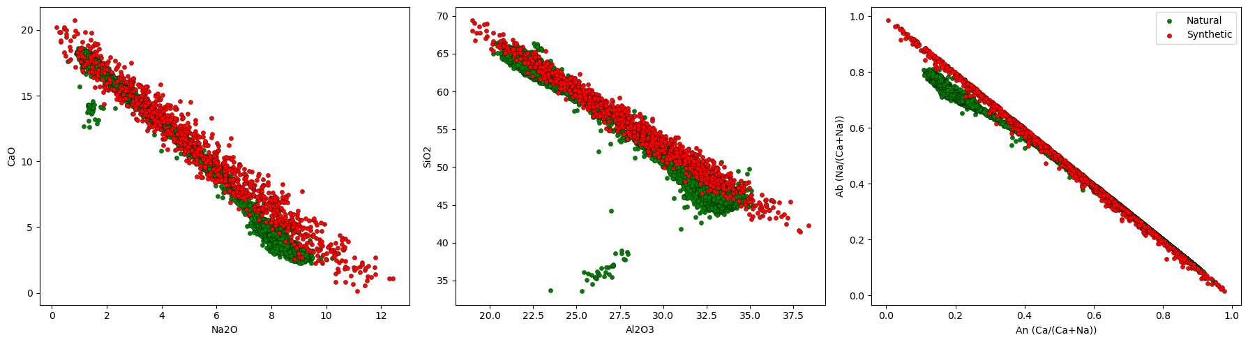
Let’s double check that this generator works, and apply this to plagioclase as a simple binary solid solution between albite (NaAlSi₃O₈) and anorthite (CaAl₂Si₂O₈). We understand plagioclase feldspar systematics quite well, so we can test this before applying this to a more complex system. We will have an 8-oxygen basis, add small amounts of K as a minor element, and then check that the synthetic cloud matches the natural data. The steps are as above.
[5]:
# Pull natural data
df_plag_natural = df_load[df_load["Mineral"]=="Plagioclase"]
plag_calc_natural = mm.FeldsparCalculator(df_plag_natural)
plag_comp_natural = plag_calc_natural.calculate_components()

# Define endmembers
plag_endmembers = {
    # Albite: NaAlSi₃O₈
    'Ab': {'Na': 1, 'Al': 1, 'Si': 3, 'O': 8},
    # Anorthite: CaAl₂Si₂O₈
    'An': {'Ca': 1, 'Al': 2, 'Si': 2, 'O': 8},
}

# Specify minor elements
plag_minors = {'K': {'distribution': 'exponential', 'scale': 0.01, 'max_fraction': 0.02}}

# Instantiate generator
plag_gen = mm.SolidSolutionGenerator(
    endmembers=plag_endmembers,
    oxygen_basis=8,
    element_noise_scale=0.05,
    min_site_fraction=0.2,
    minor_elements=plag_minors,
    mixing_dist='beta',
    mixing_params={'a': 2, 'b': 2}
)

# Generate samples
df_plag = plag_gen.generate(1000)
plag_calc_synth = mm.FeldsparCalculator(df_plag)
plag_comp_synth = plag_calc_synth.calculate_components()
display(plag_comp_synth)

# Calculate and compare the distributions of the output data
stats_pl = plag_gen.compare_distributions(base_df=plag_comp_natural, synth_df=plag_comp_synth, suptitle="Plagioclase")
display(stats_pl)

# Scatter‐plot comparing base vs. synthetic oxide proportions
fig, ax = plt.subplots(1, 3, figsize=(18, 5))
ax[0].scatter(plag_comp_natural["Na2O"], plag_comp_natural["CaO"], s=20, c="g", lw=0.25, ec='k')
ax[0].scatter(plag_comp_synth["Na2O"], plag_comp_synth["CaO"], s=20, c="r", lw=0.25, ec='k')
ax[0].set_xlabel("Na2O")
ax[0].set_ylabel("CaO")

ax[1].scatter(plag_comp_natural["Al2O3"], plag_comp_natural["SiO2"], s=20, c="g", lw=0.25, ec='k')
ax[1].scatter(plag_comp_synth["Al2O3"], plag_comp_synth["SiO2"], s=20, c="r", lw=0.25, ec='k')
ax[1].set_xlabel("Al2O3")
ax[1].set_ylabel("SiO2")

ax[2].scatter(plag_comp_natural["An"], plag_comp_natural["Ab"], s=20, c="g", lw=0.25, ec='k', label="Natural")
ax[2].scatter(plag_comp_synth["An"], plag_comp_synth["Ab"], s=20, c="r", lw=0.25, ec='k', label="Synthetic")
ax[2].set_xlabel("An (Ca/(Ca+Na))")
ax[2].set_ylabel("Ab (Na/(Ca+Na))")
ax[2].legend()
plt.tight_layout()
Charge mismatch: 17.65 vs 16
Charge mismatch: 17.64 vs 16
Charge mismatch: 14.22 vs 16
Charge mismatch: 18.35 vs 16
Charge mismatch: 14.32 vs 16
Charge mismatch: 17.83 vs 16
Charge mismatch: 14.04 vs 16
Charge mismatch: 14.03 vs 16
Charge mismatch: 18.14 vs 16
Charge mismatch: 18.18 vs 16
Charge mismatch: 18.16 vs 16
Charge mismatch: 17.81 vs 16
Charge mismatch: 13.94 vs 16
Charge mismatch: 13.87 vs 16
Charge mismatch: 18.64 vs 16
Charge mismatch: 17.90 vs 16
Charge mismatch: 17.92 vs 16
Charge mismatch: 17.71 vs 16
Charge mismatch: 14.29 vs 16
Charge mismatch: 13.88 vs 16
Charge mismatch: 17.78 vs 16
Charge mismatch: 14.40 vs 16
Charge mismatch: 14.24 vs 16
Charge mismatch: 14.31 vs 16
Charge mismatch: 17.61 vs 16
Charge mismatch: 14.36 vs 16
Charge mismatch: 14.38 vs 16
Charge mismatch: 17.87 vs 16
Charge mismatch: 17.90 vs 16
Charge mismatch: 18.10 vs 16
Charge mismatch: 17.65 vs 16
Charge mismatch: 18.08 vs 16
Charge mismatch: 17.72 vs 16
Charge mismatch: 14.38 vs 16
Charge mismatch: 13.92 vs 16
Charge mismatch: 17.68 vs 16
Charge mismatch: 13.80 vs 16
| Sample | SiO2 | Al2O3 | CaO | Na2O | K2O | SiO2_mols | Al2O3_mols | CaO_mols | Na2O_mols | ... | Prediction_Score | Prediction_Score_Sigma | Second_Predict_Mineral | Second_Prediction_Score | Cation_Sum | M_site | T_site | An | Ab | Or | |
|---|---|---|---|---|---|---|---|---|---|---|---|---|---|---|---|---|---|---|---|---|---|
| 0 | NaN | 59.460622 | 25.952514 | 5.182643 | 8.819577 | 0.584644 | 0.989691 | 0.254536 | 0.092419 | 0.142300 | ... | NaN | NaN | NaN | NaN | 5.062328 | 1.044083 | 4.018245 | 0.237319 | 0.730806 | 0.031876 |
| 1 | NaN | 64.047671 | 22.197230 | 2.714266 | 11.028512 | 0.012321 | 1.066040 | 0.217705 | 0.048402 | 0.177940 | ... | NaN | NaN | NaN | NaN | 5.062958 | 1.074603 | 3.988355 | 0.119646 | 0.879707 | 0.000647 |
| 2 | NaN | 62.040566 | 23.074472 | 4.113203 | 10.702734 | 0.069024 | 1.032633 | 0.226309 | 0.073349 | 0.172684 | ... | NaN | NaN | NaN | NaN | 5.096514 | 1.123871 | 3.972643 | 0.174564 | 0.821948 | 0.003488 |
| 3 | NaN | 53.926853 | 29.236092 | 12.578089 | 4.123420 | 0.135547 | 0.897584 | 0.286741 | 0.224299 | 0.066529 | ... | NaN | NaN | NaN | NaN | 4.970187 | 0.977686 | 3.992501 | 0.622645 | 0.369366 | 0.007989 |
| 4 | NaN | 59.268809 | 25.385215 | 6.827795 | 8.012397 | 0.505784 | 0.986498 | 0.248972 | 0.121757 | 0.129276 | ... | NaN | NaN | NaN | NaN | 5.041107 | 1.051093 | 3.990014 | 0.311360 | 0.661178 | 0.027462 |
| ... | ... | ... | ... | ... | ... | ... | ... | ... | ... | ... | ... | ... | ... | ... | ... | ... | ... | ... | ... | ... | ... |
| 995 | NaN | 59.050816 | 26.019549 | 5.518501 | 9.383394 | 0.027740 | 0.982870 | 0.255194 | 0.098409 | 0.151397 | ... | NaN | NaN | NaN | NaN | 5.084953 | 1.078119 | 4.006834 | 0.244925 | 0.753609 | 0.001466 |
| 996 | NaN | 53.598291 | 29.890896 | 10.429338 | 5.912343 | 0.169132 | 0.892115 | 0.293163 | 0.185981 | 0.095393 | ... | NaN | NaN | NaN | NaN | 5.046133 | 1.032568 | 4.013565 | 0.488964 | 0.501595 | 0.009441 |
| 997 | NaN | 51.959308 | 30.779872 | 12.255669 | 4.929267 | 0.075884 | 0.864835 | 0.301882 | 0.218549 | 0.079531 | ... | NaN | NaN | NaN | NaN | 5.038022 | 1.033939 | 4.004084 | 0.576308 | 0.419444 | 0.004249 |
| 998 | NaN | 58.209449 | 26.679834 | 9.683447 | 5.410578 | 0.016691 | 0.968866 | 0.261670 | 0.172680 | 0.087297 | ... | NaN | NaN | NaN | NaN | 4.934358 | 0.932326 | 4.002032 | 0.496737 | 0.502243 | 0.001019 |
| 999 | NaN | 59.241188 | 25.734320 | 7.480539 | 7.336771 | 0.207182 | 0.986038 | 0.252396 | 0.133397 | 0.118375 | ... | NaN | NaN | NaN | NaN | 5.002290 | 1.004402 | 3.997888 | 0.356155 | 0.632100 | 0.011745 |
1000 rows × 34 columns
(<Figure size 1200x600 with 11 Axes>,
              ks_stat        p_value  mean_base  mean_synth  std_base  \
 cation
 Si_cat_8ox  0.323833   5.514531e-89   2.427908    2.487417  0.307028
 Al_cat_8ox  0.284369   2.484052e-68   1.554179    1.510300  0.296910
 Ca_cat_8ox  0.339222   7.681478e-98   0.582427    0.508972  0.308634
 Na_cat_8ox  0.351959  1.613700e-105   0.385243    0.491474  0.268054
 K_cat_8ox   0.342515  8.537683e-100   0.028198    0.010015  0.035713

             std_synth
 cation
 Si_cat_8ox   0.229870
 Al_cat_8ox   0.233183
 Ca_cat_8ox   0.225994
 Na_cat_8ox   0.227782
 K_cat_8ox    0.010432  )
Kalsilite
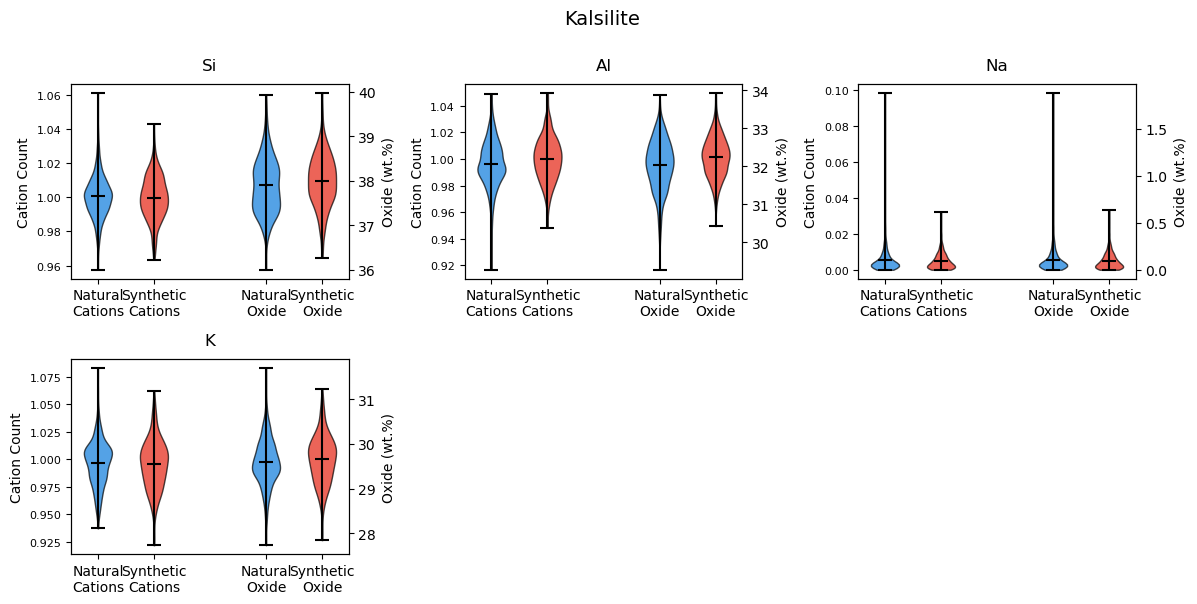
Success, this mm.SolidSolutionGenerator works with familiar solid solution minerals. Let’s test wonkier (less common) minerals, such as kalsilite. Kalsilite is a feldspathoid mineral that shares the tridymite framework. There is a Na-K exchange between nepheline and kalsilite. We will have a 4-oxygen basis and check that the synthetic cloud matches the natural data. The steps are as above.
[6]:
# Pull natural data
df_ks_natural = df_load[df_load["Mineral"]=="Kalsilite"]
ks_calc_natural = mm.KalsiliteCalculator(df_ks_natural)
ks_comp_natural = ks_calc_natural.calculate_components()
# Define endmembers
ks_endmembers = {
# Kalsilite K[AlSiO₄]
"Ks": {"K": 1, "Al": 1, "Si": 1, "O": 4},
# Nepheline Na[AlSiO₄] ~ simplification
"Ne": {"Na": 1, "Al": 1, "Si": 1, "O": 4}
}
# Specify minor elements
ks_minors = {} # no minors for pure K[AlSiO₄]-Na[AlSiO₄]
# Instantiate generator
gen_ks = mm.SolidSolutionGenerator(
endmembers = ks_endmembers,
oxygen_basis = 4,
minor_elements = ks_minors,
element_noise_scale = 0.02,
min_site_fraction = 0.2,
mixing_dist = "beta",
mixing_params = {"a": 1, "b": 200},
)
# Generate samples, use the kalsilite calculator to calculate site allocations, etc.
df_ks = gen_ks.generate(n_samples=500)
ks_calc_synth = mm.KalsiliteCalculator(df_ks)
ks_comp_synth = ks_calc_synth.calculate_components()
ks_comp_synth['Mineral'] = 'Kalsilite'
display(ks_comp_synth)
# Calculate and compare the distributions of the output data
stats_ks = gen_ks.compare_distributions(base_df=ks_comp_natural, synth_df=ks_comp_synth, suptitle="Kalsilite")
display(stats_ks)
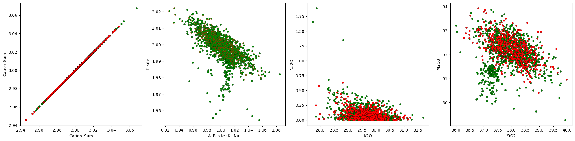
fig, ax = plt.subplots(1, 4, figsize = (20, 5))
ax = ax.flatten()
ax[0].scatter(ks_comp_natural['Cation_Sum'], ks_comp_natural['Cation_Sum'], s=20, c="g", lw=0.25, ec='k')
ax[0].scatter(ks_comp_synth['Cation_Sum'], ks_comp_synth['Cation_Sum'], s=20, c="r", lw=0.25, ec='k')
ax[0].set_xlabel('Cation_Sum')
ax[0].set_ylabel('Cation_Sum')
ax[1].scatter(ks_comp_natural['A_B_site'], ks_comp_natural['T_site'], s=20, c="g", lw=0.25, ec='k')
ax[1].scatter(ks_comp_synth['A_B_site'], ks_comp_synth['T_site'], s=20, c="g", lw=0.25, ec='r')
ax[1].set_xlabel('A_B_site (K+Na)')
ax[1].set_ylabel('T_site')
ax[2].scatter(ks_comp_natural['K2O'], ks_comp_natural['Na2O'], s=20, c="g", lw=0.25, ec='k')
ax[2].scatter(ks_comp_synth['K2O'], ks_comp_synth['Na2O'], s=20, c="r", lw=0.25, ec='k')
ax[2].set_xlabel('K2O')
ax[2].set_ylabel('Na2O')
ax[3].scatter(ks_comp_natural['SiO2'], ks_comp_natural['Al2O3'], s=20, c="g", lw=0.25, ec='k', label='Natural')
ax[3].scatter(ks_comp_synth['SiO2'], ks_comp_synth['Al2O3'], s=20, c="r", lw=0.25, ec='k', label='Synthetic')
ax[3].set_xlabel('SiO2')
ax[3].set_ylabel('Al2O3')
plt.tight_layout()
plt.show()
Charge mismatch: 9.05 vs 8
Charge mismatch: 6.78 vs 8
Charge mismatch: 9.14 vs 8
Charge mismatch: 8.90 vs 8
Charge mismatch: 8.89 vs 8
Charge mismatch: 9.05 vs 8
Charge mismatch: 8.80 vs 8
Charge mismatch: 7.09 vs 8
Charge mismatch: 8.96 vs 8
Charge mismatch: 7.13 vs 8
Charge mismatch: 7.13 vs 8
Charge mismatch: 6.90 vs 8
Charge mismatch: 9.18 vs 8
Charge mismatch: 7.06 vs 8
Charge mismatch: 7.17 vs 8
Charge mismatch: 8.84 vs 8
Charge mismatch: 8.87 vs 8
Charge mismatch: 8.84 vs 8
Charge mismatch: 8.93 vs 8
Charge mismatch: 8.95 vs 8
Charge mismatch: 8.82 vs 8
Charge mismatch: 8.85 vs 8
Charge mismatch: 7.04 vs 8
| Sample | SiO2 | Al2O3 | Na2O | K2O | SiO2_mols | Al2O3_mols | Na2O_mols | K2O_mols | SiO2_ox | ... | Predict_Mineral | Prediction_Score | Prediction_Score_Sigma | Second_Predict_Mineral | Second_Prediction_Score | Cation_Sum | A_B_site | A_site | B_site | T_site | |
|---|---|---|---|---|---|---|---|---|---|---|---|---|---|---|---|---|---|---|---|---|---|
| 0 | NaN | 39.398207 | 31.499564 | 0.151414 | 28.950815 | 0.655762 | 0.308940 | 0.002443 | 0.307347 | 1.311525 | ... | NaN | NaN | NaN | NaN | NaN | 2.971933 | 0.972600 | 0.964930 | 0.007670 | 1.999334 |
| 1 | NaN | 37.887370 | 32.515291 | 0.019159 | 29.578180 | 0.630615 | 0.318902 | 0.000309 | 0.314007 | 1.261231 | ... | NaN | NaN | NaN | NaN | NaN | 2.996622 | 0.993000 | 0.992023 | 0.000977 | 2.003622 |
| 2 | NaN | 37.966272 | 32.135924 | 0.035911 | 29.861893 | 0.631929 | 0.315182 | 0.000579 | 0.317019 | 1.263857 | ... | NaN | NaN | NaN | NaN | NaN | 3.003542 | 1.005455 | 1.003621 | 0.001834 | 1.998088 |
| 3 | NaN | 38.260329 | 32.347487 | 0.004657 | 29.387528 | 0.636823 | 0.317257 | 0.000075 | 0.311983 | 1.273646 | ... | NaN | NaN | NaN | NaN | NaN | 2.987936 | 0.983838 | 0.983601 | 0.000237 | 2.004098 |
| 4 | NaN | 36.991351 | 32.277292 | 0.002631 | 30.728727 | 0.615702 | 0.316568 | 0.000042 | 0.326221 | 1.231403 | ... | NaN | NaN | NaN | NaN | NaN | 3.033241 | 1.040974 | 1.040839 | 0.000135 | 1.992266 |
| ... | ... | ... | ... | ... | ... | ... | ... | ... | ... | ... | ... | ... | ... | ... | ... | ... | ... | ... | ... | ... | ... |
| 495 | NaN | 37.337217 | 32.480681 | 0.025390 | 30.156712 | 0.621458 | 0.318563 | 0.000410 | 0.320149 | 1.242917 | ... | NaN | NaN | NaN | NaN | NaN | 3.016399 | 1.017983 | 1.016682 | 0.001301 | 1.998416 |
| 496 | NaN | 37.672011 | 31.853838 | 0.031845 | 30.442306 | 0.627031 | 0.312415 | 0.000514 | 0.323180 | 1.254062 | ... | NaN | NaN | NaN | NaN | NaN | 3.020674 | 1.029643 | 1.028009 | 0.001634 | 1.991030 |
| 497 | NaN | 37.864325 | 32.902749 | 0.264994 | 28.967932 | 0.630232 | 0.322703 | 0.004276 | 0.307528 | 1.260464 | ... | NaN | NaN | NaN | NaN | NaN | 2.990495 | 0.981914 | 0.968450 | 0.013464 | 2.008580 |
| 498 | NaN | 38.217503 | 31.696522 | 0.261382 | 29.824593 | 0.636110 | 0.310872 | 0.004217 | 0.316623 | 1.272220 | ... | NaN | NaN | NaN | NaN | NaN | 3.008357 | 1.016250 | 1.002892 | 0.013358 | 1.992107 |
| 499 | NaN | 38.211059 | 32.335294 | 0.113227 | 29.340420 | 0.636003 | 0.317137 | 0.001827 | 0.311483 | 1.272006 | ... | NaN | NaN | NaN | NaN | NaN | 2.991093 | 0.988075 | 0.982314 | 0.005761 | 2.003018 |
500 rows × 29 columns
(<Figure size 1200x600 with 10 Axes>,
             ks_stat   p_value  mean_base  mean_synth  std_base  std_synth
 cation
 Si_cat_4ox    0.054  0.282183   1.000535    0.999837  0.012252   0.012897
 Al_cat_4ox    0.122  0.000094   0.996509    1.000027  0.017107   0.016177
 Na_cat_4ox    0.063  0.139869   0.005185    0.004836  0.006651   0.004619
 K_cat_4ox     0.060  0.178957   0.996766    0.995734  0.020745   0.022908)