This page was generated from docs/examples/mineralML_interactive.ipynb. Interactive online version: .

Python Notebook Download

""" Created on April 24, 2026 // @author: Sarah Shi """

import numpy as np
import sys
sys.path.append('../../src/')
import mineralML as mm

import matplotlib.pyplot as plt
%matplotlib inline
%config InlineBackend.figure_format = 'png'

Interactive Tools for Mapped EDS Data

This notebook demonstrates interactive tools for exploring mineralML phase maps. These tools require a live Python kernel and an interactive Matplotlib backend — they cannot be run on ReadTheDocs. Use the Colab badge above or run locally with %matplotlib widget (requires ipympl).

pip install ipympl

The tools shown here are:

• ``mm.interactive_pixels`` — click pixels to sample oxide compositions

• ``mm.interactive_line_profile`` — click to draw transects and extract line profiles

• ``mm.plot_locations`` — plot the locations of picked pixels or transects on a map

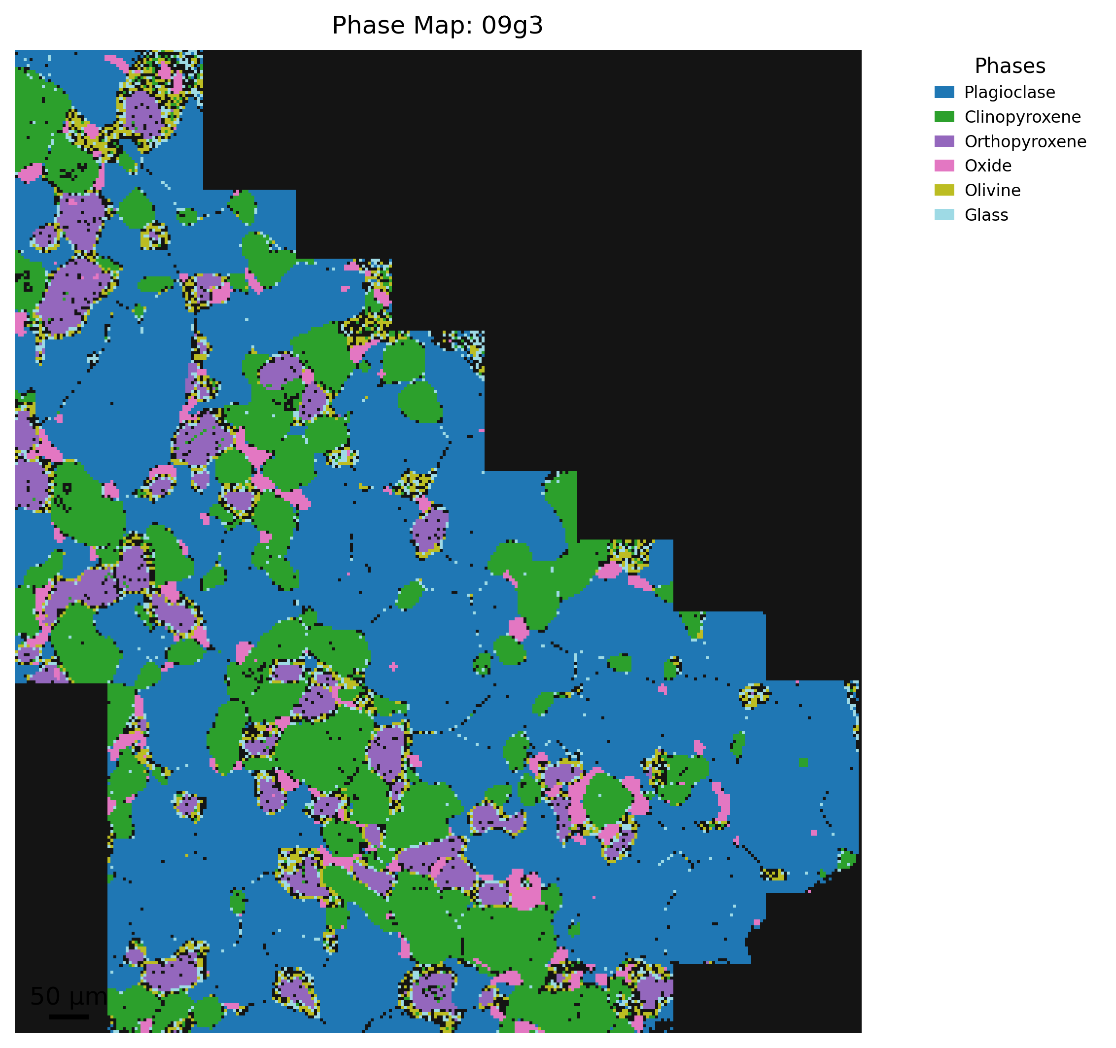
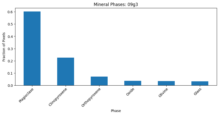
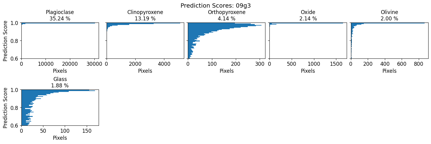
1. Load and run a map

First, run mm.run_map as usual to get the result dictionary. See the EDS mapping notebook for full details on loading and preparing data.

%matplotlib inline

result = mm.run_map(
    "Maps/09g3",
    renormalize=True,
    units="element_wt%",
    pixel_size_um=4.0,
    scalebar_um=50,
    total_threshold=50,
    min_frac=0.01,
)

[ok] Mg Wt%Montaged Map Data.csv  →  Mg  (329, 283)
[ok] Ca Wt%Montaged Map Data.csv  →  Ca  (329, 283)
[ok] Al Wt%Montaged Map Data.csv  →  Al  (329, 283)
[ok] Fe Wt%Montaged Map Data.csv  →  Fe  (329, 283)
[ok] Na Wt%Montaged Map Data.csv  →  Na  (329, 283)
[ok] Mn Wt%Montaged Map Data.csv  →  Mn  (329, 283)
[ok] Cr Wt%Montaged Map Data.csv  →  Cr  (329, 283)
[ok] Ti Wt%Montaged Map Data.csv  →  Ti  (329, 283)
[ok] Si Wt%Montaged Map Data.csv  →  Si  (329, 283)
[ok] K Wt%Montaged Map Data.csv  →  K  (329, 283)
mineralML: 93107 rows — 57732 classified by neural network, 0 by empirical rules (Zircon: 0, SiO2 polymorph: 0, Carbonate: 0), 35375 skipped (invalid/empty)
prep_df: 57732 row(s) processed (of 57732 input, 0 dropped).

/Users/sarahshi/Documents/GitHub/mineralML/docs/examples/../../src/mineralML/hybrid.py:280: UserWarning: The column 'Mineral' was missing and has been filled with NaN.
  df = prep_df(df)
/Users/sarahshi/Documents/GitHub/mineralML/docs/examples/../../src/mineralML/hybrid.py:280: UserWarning: Non-numeric values in 57732 row(s) were coerced to NaN.
  df = prep_df(df)

2. Interactive pixel composition picker

mm.interactive_pixels displays the phase map and records the full oxide composition of each pixel you click. Each click:

• Places a marker on the map

• Prints the oxide values below the figure

• Appends a row to the dataframe in controller["picks"]

Keybindings: r/u undo last pick  |  c clear all  |  q/Esc quit

After quitting, access your picks as a DataFrame:

controller["picks"]

%matplotlib widget

controller = mm.interactive_pixels(result,
                                   region=3, # side length of square averaging box (1 = single pixel; use odd integers, e.g. 3, 5)
                                   phase=None, # specify phase to display (e.g. "plagioclase"); if None, will display all pixels regardless of phase assignment
                                   )

%matplotlib inline

controller["picks"]

	x	y	phase	n_pixels	SiO2	TiO2	Al2O3	FeOt	MnO	MgO	CaO	Na2O	K2O	Cr2O3	Total	Total_raw
0	24	74	Orthopyroxene	9	51.382158	0.231275	5.935667	14.527422	0.092448	26.585354	0.838933	0.338983	-0.013140	0.080898	100.0	99.452320
1	14	85	Orthopyroxene	9	51.755858	0.266427	6.422178	13.811186	0.208105	26.407858	0.979675	0.164893	-0.041242	0.025062	100.0	99.796230
2	41	107	Plagioclase	9	51.243466	0.164586	31.054675	0.062434	-0.078979	-0.104385	13.301734	4.251682	0.276118	-0.171331	100.0	98.990366
3	38	128	Plagioclase	9	52.196867	-0.024729	30.320998	0.405566	-0.004646	0.046737	12.551467	4.307204	0.332112	-0.131575	100.0	98.874299
4	95	232	Clinopyroxene	9	49.447336	0.722313	8.024595	6.979877	0.101082	13.946927	19.894387	0.797412	0.256247	-0.170175	100.0	97.394634
5	103	240	Clinopyroxene	9	49.604274	0.561800	8.036716	6.500822	0.003462	13.893682	20.402058	0.840622	0.130585	0.025979	100.0	99.288592
6	168	283	Oxide	9	-0.048897	0.267502	59.991736	22.327466	-0.148192	15.930729	0.118597	0.117541	0.018457	1.425061	100.0	97.400370
7	173	283	Oxide	9	-0.249181	0.119954	60.926417	21.555273	-0.020259	16.497383	0.043414	-0.083181	-0.017739	1.227919	100.0	98.294721

2a. Filter to a specific phase

Pass phase to restrict the display and clicks to one or more mineral phases. Pixels outside the selected phase are shown as white background.

%matplotlib widget

controller_opx = mm.interactive_pixels(result,
                                       region=3, # side length of square averaging box (1 = single pixel; use odd integers, e.g. 3, 5)
                                       phase="Plagioclase" # plot only pixels classified as plagioclase (optional; if None, will display all pixels regardless of phase assignment
                                       )

2b. Display an oxide heatmap as background

Pass oxide_key to show an oxide or component concentration map instead of the phase map. Combine with phase to restrict to a single mineral.

%matplotlib widget

controller_sio2 = mm.interactive_pixels(result,
                                        region=3, # side length of square averaging box (1 = single pixel; use odd integers, e.g. 3, 5)
                                        oxide_key="Feldspar.An", # plot An content of each pixel instead of phase assignment
                                        phase="Plagioclase" # plot only pixels classified as plagioclase (optional; if None, will display all pixels regardless of phase assignment
                                        )

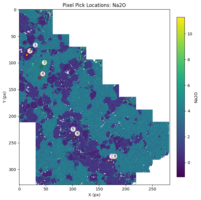
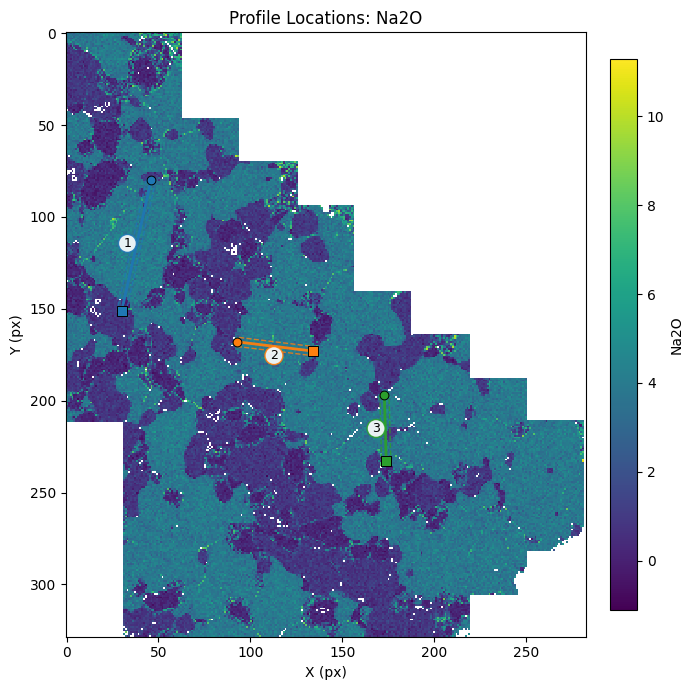
3. Plot pick locations

mm.plot_locations overlays picked pixel locations on a map. Pass map_key to use an oxide map as the background.

%matplotlib inline

fig, ax = mm.plot_locations(result,
                            controller["picks"], # plot only the pixels that have been picked
                            map_key="Na2O", # color the points by their Na2O content
                            )

4. Interactive line profiles

mm.interactive_line_profile lets you draw transects across a map by clicking a start and end point. Each completed transect is extracted and plotted immediately.

Keybindings: r reset current clicks  |  u undo last transect  |  c clear all  |  q/Esc quit

Access results after quitting:

lp["profiles_df"]     # all profile data concatenated
lp["coordinates_df"]  # transect start/end coordinates

%matplotlib widget

lp = mm.interactive_line_profile(
    result,
    key="SiO2", # key of the oxide map to plot the line profile for
    method="none", # do not apply any smoothing to the line profile. use mean or median (across the pixel width) for a smoothed profile
    width_px=5, # width of the line profile in pixels
    pixel_size_um=4.0, # pixel size in micrometers
)

4a. Filter transects to a single phase

Pass phase to mask the background map to pixels of a specific mineral before drawing transects.

%matplotlib widget

lp_opx = mm.interactive_line_profile(
    result,
    key="Feldspar.An", # plot the Mg# of pixels classified as plagioclase
    phase="Plagioclase",
    method="none",
    width_px=5,
    pixel_size_um=4.0,
)

Return the line profile dataframe.

%matplotlib inline

lp["profiles_df"]

	profile_id	distance_px	distance_um	SiO2	SiO2_smoothed	x	y	perp_distance_px	source	width_px	length_px	length_um	color	x0	y0	x1	y1
0	1	0.029312	0.117246	49.490084	49.490084	46.0	80.0	0.452090	auto	5.0	72.893565	291.574258	#1f77b4	46	80	30	151
1	1	0.254171	1.016684	48.257454	48.257454	45.0	80.0	1.426481	auto	5.0	72.893565	291.574258	#1f77b4	46	80	30	151
2	1	0.479031	1.916122	50.015794	50.015794	44.0	80.0	2.400872	auto	5.0	72.893565	291.574258	#1f77b4	46	80	30	151
3	1	0.553984	2.215935	40.963464	40.963464	48.0	81.0	-1.721552	auto	5.0	72.893565	291.574258	#1f77b4	46	80	30	151
4	1	0.778843	3.115373	53.601392	53.601392	47.0	81.0	-0.747161	auto	5.0	72.893565	291.574258	#1f77b4	46	80	30	151
...	...	...	...	...	...	...	...	...	...	...	...	...	...	...	...	...	...
750	3	36.333159	145.332637	51.627654	51.627654	172.0	233.0	1.929236	auto	5.0	36.435405	145.741620	#2ca02c	173	197	174	233
751	3	36.358151	145.432606	60.081533	60.081533	173.0	233.0	0.929548	auto	5.0	36.435405	145.741620	#2ca02c	173	197	174	233
752	3	36.383144	145.532574	56.881043	56.881043	174.0	233.0	-0.070139	auto	5.0	36.435405	145.741620	#2ca02c	173	197	174	233
753	3	36.408136	145.632543	49.347756	49.347756	175.0	233.0	-1.069827	auto	5.0	36.435405	145.741620	#2ca02c	173	197	174	233
754	3	36.433128	145.732512	52.350107	52.350107	176.0	233.0	-2.069515	auto	5.0	36.435405	145.741620	#2ca02c	173	197	174	233

755 rows × 17 columns

5. Plot transect locations

Pass the coordinates_df from a line profile controller to mm.plot_locations to visualize transect positions.

%matplotlib inline

fig, ax = mm.plot_locations(result,
                            lp["coordinates_df"],
                            map_key="Na2O"
                            )

6. Batch extract profiles from saved transects

mm.batch_extract_line_profiles extracts profiles for multiple oxides at once from a saved transect table. Pass lp["coordinates_df"] from an interactive session, or any DataFrame with x0, y0, x1, y1 columns.

Each oxide becomes its own column, making it easy to compare compositions along the same transect.

%matplotlib inline

profiles_df = mm.batch_extract_line_profiles(
    result,
    transects=lp["coordinates_df"],
    keys=["SiO2", "Al2O3", "FeOt", "MgO", "CaO", "Feldspar.An"],
    method="none",
    pixel_size_um=4.0,
)

profiles_df

	profile_id	x	y	distance_px	perp_distance_px	distance_um	SiO2	SiO2_smoothed	Al2O3	Al2O3_smoothed	...	CaO	CaO_smoothed	Feldspar.An	Feldspar.An_smoothed	x0	y0	x1	y1	width_px	source
0	1	46.0	80.0	0.000000	0.000000e+00	0.000000	49.490084	49.490084	7.699435	7.699435	...	21.724662	21.724662	NaN	NaN	46.0	80.0	30.0	151.0	5.0	auto
1	1	45.0	80.0	0.219839	9.755361e-01	0.879357	48.257454	48.257454	8.595989	8.595989	...	19.916674	19.916674	NaN	NaN	46.0	80.0	30.0	151.0	5.0	auto
2	1	44.0	80.0	0.439678	1.951072e+00	1.758713	50.015794	50.015794	8.705449	8.705449	...	20.377495	20.377495	NaN	NaN	46.0	80.0	30.0	151.0	5.0	auto
3	1	48.0	81.0	0.535858	-2.170911e+00	2.143432	40.963464	40.963464	8.341098	8.341098	...	2.822591	2.822591	NaN	NaN	46.0	80.0	30.0	151.0	5.0	auto
4	1	47.0	81.0	0.755697	-1.195375e+00	3.022788	53.601392	53.601392	28.690880	28.690880	...	10.621687	10.621687	0.547575	0.547575	46.0	80.0	30.0	151.0	5.0	auto
...	...	...	...	...	...	...	...	...	...	...	...	...	...	...	...	...	...	...	...	...	...
746	3	175.0	232.0	35.042039	-1.027381e+00	140.168155	50.870222	50.870222	32.378985	32.378985	...	13.190178	13.190178	0.675179	0.675179	173.0	197.0	174.0	233.0	5.0	auto
747	3	176.0	232.0	35.069806	-2.026996e+00	140.279224	52.350337	52.350337	30.086376	30.086376	...	13.510627	13.510627	0.654615	0.654615	173.0	197.0	174.0	233.0	5.0	auto
748	3	172.0	233.0	35.958352	1.999229e+00	143.833408	51.627654	51.627654	30.454367	30.454367	...	10.819728	10.819728	0.499965	0.499965	173.0	197.0	174.0	233.0	5.0	auto
749	3	173.0	233.0	35.986119	9.996144e-01	143.944477	60.081533	60.081533	22.631185	22.631185	...	6.053288	6.053288	NaN	NaN	173.0	197.0	174.0	233.0	5.0	auto
750	3	174.0	233.0	36.013886	-5.551115e-17	144.055545	56.881043	56.881043	25.929915	25.929915	...	8.147010	8.147010	0.367105	0.367105	173.0	197.0	174.0	233.0	5.0	auto

751 rows × 24 columns

# Long format — one row per oxide per distance bin, useful for plotting
profiles_df, profiles_long_df = mm.batch_extract_line_profiles(
    result,
    transects=lp["coordinates_df"],
    keys=["SiO2", "MgO", "CaO"],
    method="mean",
    pixel_size_um=4.0,
    return_long=True,
)

profiles_long_df

	bin	distance_px	value	n_pixels	distance_um	value_smoothed	profile_id	key	source	x0	y0	x1	y1	width_px
0	0	0.099427	49.490084	1	0.397708	49.490084	1	SiO2	auto	46.0	80.0	30.0	151.0	5.0
1	1	0.298281	48.257454	1	1.193123	48.257454	1	SiO2	auto	46.0	80.0	30.0	151.0	5.0
2	2	0.497135	45.489629	2	1.988538	45.489629	1	SiO2	auto	46.0	80.0	30.0	151.0	5.0
3	3	0.695988	53.601392	1	2.783953	53.601392	1	SiO2	auto	46.0	80.0	30.0	151.0	5.0
4	4	0.894842	50.561281	1	3.579368	50.561281	1	SiO2	auto	46.0	80.0	30.0	151.0	5.0
...	...	...	...	...	...	...	...	...	...	...	...	...	...	...
2260	180	35.137873	13.350402	2	140.551491	13.350402	3	CaO	auto	173.0	197.0	174.0	233.0	5.0
2261	181	35.332542	NaN	0	141.330170	NaN	3	CaO	auto	173.0	197.0	174.0	233.0	5.0
2262	182	35.527212	NaN	0	142.108848	NaN	3	CaO	auto	173.0	197.0	174.0	233.0	5.0
2263	183	35.721882	NaN	0	142.887527	NaN	3	CaO	auto	173.0	197.0	174.0	233.0	5.0
2264	184	35.916551	8.340008	3	143.666206	8.340008	3	CaO	auto	173.0	197.0	174.0	233.0	5.0

2265 rows × 14 columns

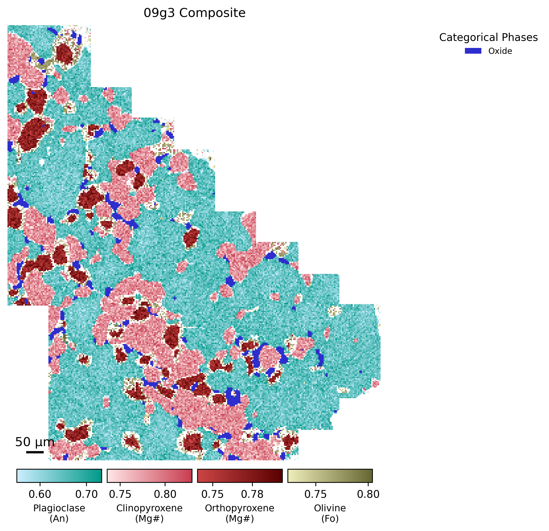
7. Composite component map

mm.plot_component_composite overlays continuous solid-solution compositions (e.g. plagioclase An%, olivine Fo%, pyroxene XMg) on top of a categorical phase map. This gives a single figure showing both phase identity and mineral chemistry.

The component maps are computed automatically by run_map and stored in result["component_maps"].

%matplotlib inline
# You can restrict which phases appear and adjust the color limits. `limits_mode="std"` clips the colorbar to the 2 sigma range of each component, which is useful when a few extreme pixels would otherwise compress the color scale.

fig, mineral_map, comp_maps = mm.plot_component_composite(
    result,
    title="09g3 Composite",
    pixel_size_um=4.0,
    scalebar_um=50,
    limits_mode="std", # 2 sigma range for color limits
)