This page was generated from
docs/examples/mineralML_mapping_ebsd.ipynb.
Interactive online version:
![]() .
.
[1]:
""" Created on March 28, 2026 // @author: Sarah Shi """

import os
import numpy as np
import pandas as pd

import mineralML as mm

import matplotlib.pyplot as plt
%matplotlib inline
%config InlineBackend.figure_format = 'png'
mineralML Quickstart for Mapped EBSD and/or EDS Data
This notebook shows how to load and run your quantitative EDS and EBSD data through mineralML with an example Mount Hood andesite: MH0811b. These data were collected for the mineralML manuscript (find the preprint here: https://doi.org/10.31223/X53J2M) and the data are in the GitHub repository (https://github.com/sarahshi/mineralML/tree/main/docs/examples/Maps/MountHood_MH0811b). Please refer to the paper for more information about this sample. The previous example workbook highlights
how EDS maps are processed. We will apply the same procedure here, but additionally highlight how the EBSD processing code for CTF files works in mineralML.
This is a seven step process:
Load and plot a phase map directly from an EBSD CTF file.
Load a directory containing all your CSVs of mapped chemical data with
mm.load_df(orpd.read_csvdirectly). [Optional] Convert the input from element to oxide wt%.Predict the mineral class with mineralML and automatically plot the mineral phase map, mineral phase counts, and prediction score histograms.
Plot EBSD and mineralML-generated EDS maps side-by-side.
Plot prediction score map and individual oxide maps.
Plot compositions of mapped minerals in various classification diagrams (ternary, quadrilateral).
Plot chemical variation maps.
I have conveniently (I hope!) wrapped all of these bits into one function, called mm.run_map and mm.plot_ctf_phases.
We loaded in the mineralML Python package as mm. mineralML has trained machine learning models for classifying minerals. This implementation aims to get your electron microprobe or quantitative EDS compositions classified and processed. We remove some degrees of freedom to simplify the process as much as possible. The minerals considered for this study include: Amphibole, Apatite, Biotite, Calcite, Chlorite, Epidote, Feldspar (Alkali Feldspar and Plagioclase), Garnet, Glass,
Kalsilite, Leucite, Melilite, Muscovite, Nepheline, Olivine, Oxide (Rhombohedral_Oxides including Hematite-Ilmenite, Spinel_Group including Magnetite-Spinel), Pyroxene (Clinopyroxene, Orthopyroxene, Na-Pyroxene), Quartz, Rutile, Serpentine, Titanite, Tourmaline, and Zircon.
CSV files containing your mapped data in oxide weight percentages (or converted to) is necessary. Find an example here. The necessary oxides are SiO\(_2\), TiO\(_2\), Al\(_2\)O\(_3\), FeO\(_t\), MnO, MgO, CaO, Na\(_2\)O, K\(_2\)O, Cr\(_2\)O\(_3\), P\(_2\)O\(_5\), and ZrO\(_2\) (if you are aiming to classify zircon). For the oxides not analyzed for specific minerals, the preprocessing will fill in the nan values as 0.
1. Load and plot a phase map from an EBSD CTF file
[2]:
# --- MH0811b Configs ---
mh_file_path = "Maps/MH0811b_EBSD_EDS.ctf" # path to the CTF file exported from AZtec

# Merge more verbose EBSD phase names into broader mineral groups, matching with mineralML naming convention
mh_merge_rules = {
    "Andesine": "Plagioclase", "Orthoclase": "Alkali_Feldspar", # feldspar endmembers to group names
    "Augite": "Clinopyroxene", "Enstatite": "Orthopyroxene", # pyroxene endmembers to group names
    "Magnetite": "Oxide", "Ilmenite": "Oxide", # Fe-Ti oxides to single oxide group
    "Quartz-new": "SiO2_Polymorph", "Cristobalite": "SiO2_Polymorph", # silica phases to single group
}

# Pin each mineral group to a consistent color across figures
mh_base_cols = {
    "Plagioclase": "#66C4C4", "Alkali_Feldspar": "#FEF7C2", "Feldspar_Miscibility_Gap": "#003D36",
    "Clinopyroxene": "#E57A7A", "Orthopyroxene": "#931D1D",
    "Oxide": "#2E2DCE", "Glass": "#F9C300",
    "Apatite": "#5B6768", "SiO2_Polymorph": "#CEC6CD",
    "Unindexed": "#FFFFFF" # white background for unindexed pixels
}
[3]:
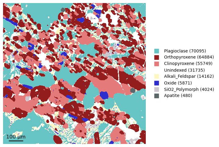
# Plot the EBSD phase map from the CTF file. This parses the CTF header for
# grid dimensions and phase definitions, maps each pixel's phase ID to its
# name, applies rename_dict for partial case-insensitive matching, and plots
# a 2D categorical phase map with legend ordered by abundance.

mh_ebsd_fig, mh_ebsd_phase_map, _, _, _ = mm.plot_ctf_phases(mh_file_path, # load and plot the CTF phase map
                                                             rename_dict=mh_merge_rules, # apply the merge rules defined above
                                                             phase_colors=mh_base_cols, # apply the color scheme defined above
                                                             title=None, # suppress the auto-generated title
                                                             scalebar_um=100, # 100 µm scale bar, computed from CTF step size
                                                             )
[4]:
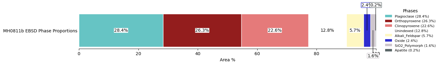
# Plot a stacked horizontal bar showing area proportions of each phase,
# normalized to classified pixels only. Phases below min_frac are excluded,
# and each segment is annotated with its percentage by default.

fig = mm.plot_phase_proportions(mh_ebsd_phase_map, # input the EBSD phase map to compute proportions
                                title="MH0811b EBSD Phase Proportions", # provide a title
                                min_frac=0.0001, # set a minimum fraction threshold to exclude very rare phases
                                phase_colors=mh_base_cols, # apply the same color scheme as the phase map
                                annotate=True, # annotate each segment with its percentage
                                )
The remaining steps are the same procedure detailed in the first mapping .ipynb on Read The Docs. We will go through it again here for reference, so we can make side by side figures.
2. Load and prepare EDS data for analysis
Here, we will work with EDS data that are in elemental weight percent. This means that we will have to do a conversion to oxide weight percent. The data directory is Maps/MountHood_MH0811b.
[5]:
# Find your directory of mapped mineral data, stored in Maps/MountHood_MH0811b.
# This code identifies any file with CSV and appends it to the map.

base = "Maps"
map_dirs = []
for root, subdirs, files in os.walk(base):
    # Skip any path that includes 'Ignore' in its folder names
    if "Ignore" in root.split(os.sep):
        continue

    if any(f.lower().endswith(".csv") for f in files):
        map_dirs.append(root)

print(map_dirs)
['Maps/09g3', 'Maps/MountHood_MH0811b']
3. Apply the trained neural network with mm.run_map
We will use mm.run_map which will return all you need!
[6]:
# Inspect the inputs and outputs of mm.run_map
help(mm.run_map)
Help on function run_map in module mineralML.mapping:

run_map(sample_input, renormalize=False, total_threshold=None, n_iterations=50, min_frac=1e-05, pred_score_threshold=0.6, units='element_wt%', top_k=None, phases=None, exclude_phases=None, phase_colors=None, bar_style='vertical', components_spec=None, remove_islands_flag=False, fill_holes_flag=False, hole_size=10, scalebar_um=None, pixel_size_um=None, scalebar_loc='lower left', scalebar_col='black', show=True)
    Load, convert, predict, and plot for one folder of CSV maps.
    Always computes mineral components and returns a full results dictionary.
    Use ``remove_islands_flag`` and ``fill_holes_flag`` to clean the phase map
    before plotting and downstream analysis.

    Parameters:
        sample_input (str | Path | dict): Directory path or a dict of oxide maps.
        renormalize (bool): If True, scale each pixel so oxides sum to 100 wt%.
            Applied after total masking.
        total_threshold (float | None): Pixels with oxide total below this
            value (wt%) are set to NaN before renormalization and prediction.
            Use this to mask epoxy/background.
        n_iterations (int): MC forward passes for prediction.
        min_frac (float): Minimum pixel fraction required to keep a phase.
        pred_score_threshold (float): Label NaN where max prediction score <
            threshold.
        units (str): Input format — 'element_wt%' or 'oxide_wt%'.
        top_k (int|None): Cap displayed phases after filtering.
        phases (list[str]|None): Explicit phases to plot (overrides auto-pick).
        exclude_phases (list[str]|None): Phases to remove from auto-pick.
        phase_colors (dict|None): Manual color mapping {PhaseName: HexColor}.
        bar_style (str): "vertical" for the default bar chart
            (``plot_phase_counts``), or "stacked" for a stacked horizontal
            bar (``plot_phase_proportions``).
        components_spec (dict|None): Custom mineral formula logic.
        remove_islands_flag (bool): If True, removes isolated pixel clusters
            smaller than 2 pixels (4-connected) from the phase map. Useful
            for cleaning up salt-and-pepper noise in the epoxy region.
        fill_holes_flag (bool): If True, fills enclosed background holes within
            continuous phase regions up to ``hole_size`` pixels. Useful for
            patching small gaps inside large mineral grains.
        hole_size (int): Maximum hole area (in pixels) to fill when
            ``fill_holes_flag`` is True.
        scalebar_um (float, optional): Length of the scale bar in micrometers.
        pixel_size_um (float): Physical size of a single pixel in micrometers.
        scalebar_loc (str): Location of the scale bar (e.g., 'lower left').
        scalebar_col (str): Color of the scale bar text/line.
        show (bool): If True, calls plt.show().

    Returns:
        result (dict): Dictionary with keys 'figs', 'shape', 'oxide_maps',
            'df_pred', 'mineral_map', 'pred_score_map', 'kept_phases',
            'component_maps', 'component_frames'. ``oxide_maps`` includes a
            ``'Total'`` key with the per-pixel oxide sum.
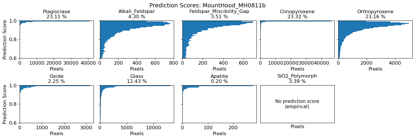
[7]:
# Here is our all in one function! Read the inputs and outputs provided above.

output = mm.run_map(next((s for s in map_dirs if 'MountHood_MH0811b' in s), None), # provide the directory of interest
                    renormalize=True, # optionally renormalize totals to 100 wt%
                    total_threshold=None, # optionally filter out total values below a given value, for when EDS picks up epoxy pixels
                    pred_score_threshold=0.6, # provide a prediction score threshold. here, i only want values with >= 0.6 prediction score
                    min_frac=0.001, # provide a minimum pixel fraction for the phase to be displayed
                    units='element_wt%', # provide the unit. can choose 'element_wt%' or 'oxide_wt%'
                    phases=mh_base_cols.keys(), # phases of interest
                    scalebar_um=100, # define size of scalebar desired, in microns
                    pixel_size_um=2.0, # define size of each pixel of scalebar, in microns
                    scalebar_loc='lower left', # specify location for scalebar
                    scalebar_col='black', # specify color for scalebar
                    phase_colors=mh_base_cols, # provide a color scheme for the phases, as a dictionary mapping phase names to color codes
                    )
[ok] MH0811b_singleframe_quant-Si Wt%.csv  →  Si  (494, 501)
[ok] MH0811b_singleframe_quant-Al Wt%.csv  →  Al  (494, 501)
[skip] no element token in: MH0811b_singleframe_quant-Sr Wt%.csv
[skip] no element token in: MH0811b_singleframe_quant-Cu Wt%.csv
[ok] MH0811b_singleframe_quant-Ni Wt%.csv  →  Ni  (494, 501)
[ok] MH0811b_singleframe_quant-Mn Wt%.csv  →  Mn  (494, 501)
[skip] no element token in: MH0811b_singleframe_quant-Cl Wt%.csv
[ok] MH0811b_singleframe_quant-Ti Wt%.csv  →  Ti  (494, 501)
[skip] no element token in: MH0811b_singleframe_quant-O Wt%.csv
[ok] MH0811b_singleframe_quant-Na Wt%.csv  →  Na  (494, 501)
[ok] MH0811b_singleframe_quant-P Wt%.csv  →  P  (494, 501)
[skip] no element token in: MH0811b_singleframe_quant-F Wt%.csv
[ok] MH0811b_singleframe_quant-K Wt%.csv  →  K  (494, 501)
[ok] MH0811b_singleframe_quant-Mg Wt%.csv  →  Mg  (494, 501)
[skip] no element token in: MH0811b_singleframe_quant-S Wt%.csv
[ok] MH0811b_singleframe_quant-Fe Wt%.csv  →  Fe  (494, 501)
[ok] MH0811b_singleframe_quant-Ca Wt%.csv  →  Ca  (494, 501)
[ok] MH0811b_singleframe_quant-Cr Wt%.csv  →  Cr  (494, 501)
mineralML: 247494 rows — 238609 classified by neural network, 8390 by empirical rules (Zircon: 0, SiO2 polymorph: 8390, Carbonate: 0), 495 skipped (invalid/empty)
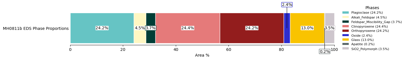
[8]:
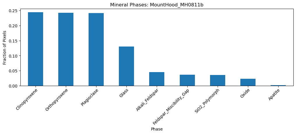
# Plot a stacked horizontal bar showing area proportions of each phase,
# normalized to classified pixels only. Phases below min_frac are excluded,
# and each segment is annotated with its percentage by default.

fig = mm.plot_phase_proportions(output['mineral_map'], # input the EDS phase map to compute proportions
                                title="MH0811b EDS Phase Proportions", # provide a title
                                phases=mh_base_cols.keys(), # specify the phases to include
                                min_frac=0.0001, # set a minimum fraction threshold to exclude very rare phases
                                phase_colors=mh_base_cols, # apply the same color scheme as the phase map
                                annotate=True, # annotate each segment with its percentage
                                )
[9]:
# Inspect what is in the outputs
output.keys()
[9]:
dict_keys(['figs', 'shape', 'oxide_maps', 'df_pred', 'mineral_map', 'pred_score_map', 'kept_phases', 'component_maps', 'component_frames'])
Let’s say you now want to work with these data in dataframe form rather than dictionary form. How would you do this? Access output['df_pred'] to retrieve the predictions dataframe.
[10]:
# Pull the dataframe of predictions
df_pred = output['df_pred']
display(df_pred)
| SiO2 | TiO2 | Al2O3 | FeOt | MnO | MgO | CaO | Na2O | K2O | Cr2O3 | P2O5 | ZrO2 | Predict_Mineral | Prediction_Score | Prediction_Score_Sigma | Second_Predict_Mineral | Second_Prediction_Score | Submineral | |
|---|---|---|---|---|---|---|---|---|---|---|---|---|---|---|---|---|---|---|
| 0 | 52.869693 | 0.089446 | 1.409243 | 21.357081 | 0.382089 | 21.732924 | 1.831746 | 0.069385 | 0.182859 | 0.000000 | 0.000000 | NaN | Orthopyroxene | 0.954259 | 0.121515 | Amphibole | 0.045181 | Enstatite |
| 1 | 51.892819 | 0.591858 | 1.289309 | 22.414176 | 1.120519 | 20.739631 | 1.453647 | 0.155577 | 0.000000 | 0.000000 | 0.000000 | NaN | Orthopyroxene | 0.926802 | 0.161589 | Amphibole | 0.072842 | Enstatite |
| 2 | 52.287424 | 0.306354 | 0.442857 | 22.273798 | 0.656842 | 21.441527 | 1.709473 | 0.313483 | 0.159156 | 0.326132 | 0.000000 | NaN | Orthopyroxene | 0.937167 | 0.156033 | Amphibole | 0.053794 | Enstatite |
| 3 | 51.667645 | 0.468977 | 1.602369 | 23.606152 | 0.000000 | 20.711076 | 1.316344 | 0.364752 | 0.000000 | 0.000000 | 0.000000 | NaN | Orthopyroxene | 0.868075 | 0.213352 | Amphibole | 0.130258 | Enstatite |
| 4 | 53.113961 | 0.000000 | 1.850691 | 22.954577 | 0.603992 | 19.687578 | 1.703375 | 0.000000 | 0.078555 | 0.007271 | 0.000000 | NaN | Orthopyroxene | 0.955211 | 0.083039 | Amphibole | 0.041217 | Enstatite |
| ... | ... | ... | ... | ... | ... | ... | ... | ... | ... | ... | ... | ... | ... | ... | ... | ... | ... | ... |
| 247489 | 75.658296 | 0.020106 | 2.377803 | 10.960863 | 0.761252 | 7.599581 | 0.830684 | 0.574031 | 0.352833 | 0.168437 | 0.288810 | NaN | Glass | 0.999502 | 0.002028 | Amphibole | 0.000485 | NaN |
| 247490 | 52.781085 | 0.000000 | 1.084068 | 25.244632 | 0.585867 | 18.465076 | 1.386827 | 0.436795 | 0.000000 | 0.000000 | 0.015651 | NaN | Orthopyroxene | 0.800574 | 0.286466 | Amphibole | 0.195758 | Enstatite |
| 247491 | 52.136743 | 0.332666 | 0.759727 | 23.384690 | 0.000000 | 21.442475 | 1.262017 | 0.000000 | 0.000000 | 0.573398 | 0.000000 | NaN | Orthopyroxene | 0.955728 | 0.141057 | Amphibole | 0.043054 | Enstatite |
| 247492 | 52.276311 | 0.283907 | 1.219325 | 21.488206 | 0.775673 | 21.428622 | 1.410546 | 0.323923 | 0.107557 | 0.174155 | 0.000000 | NaN | Orthopyroxene | 0.762849 | 0.309576 | Amphibole | 0.236592 | Enstatite |
| 247493 | NaN | NaN | NaN | NaN | NaN | NaN | NaN | NaN | NaN | NaN | NaN | NaN | None | NaN | NaN | NaN | NaN | NaN |
247494 rows × 18 columns
4. Plot EBSD and mineralML-generated EDS phase maps side-by-side
Let’s plot the two phase maps side by side!
[11]:
# EBSD phase map
mh_ebsd_fig
[11]:

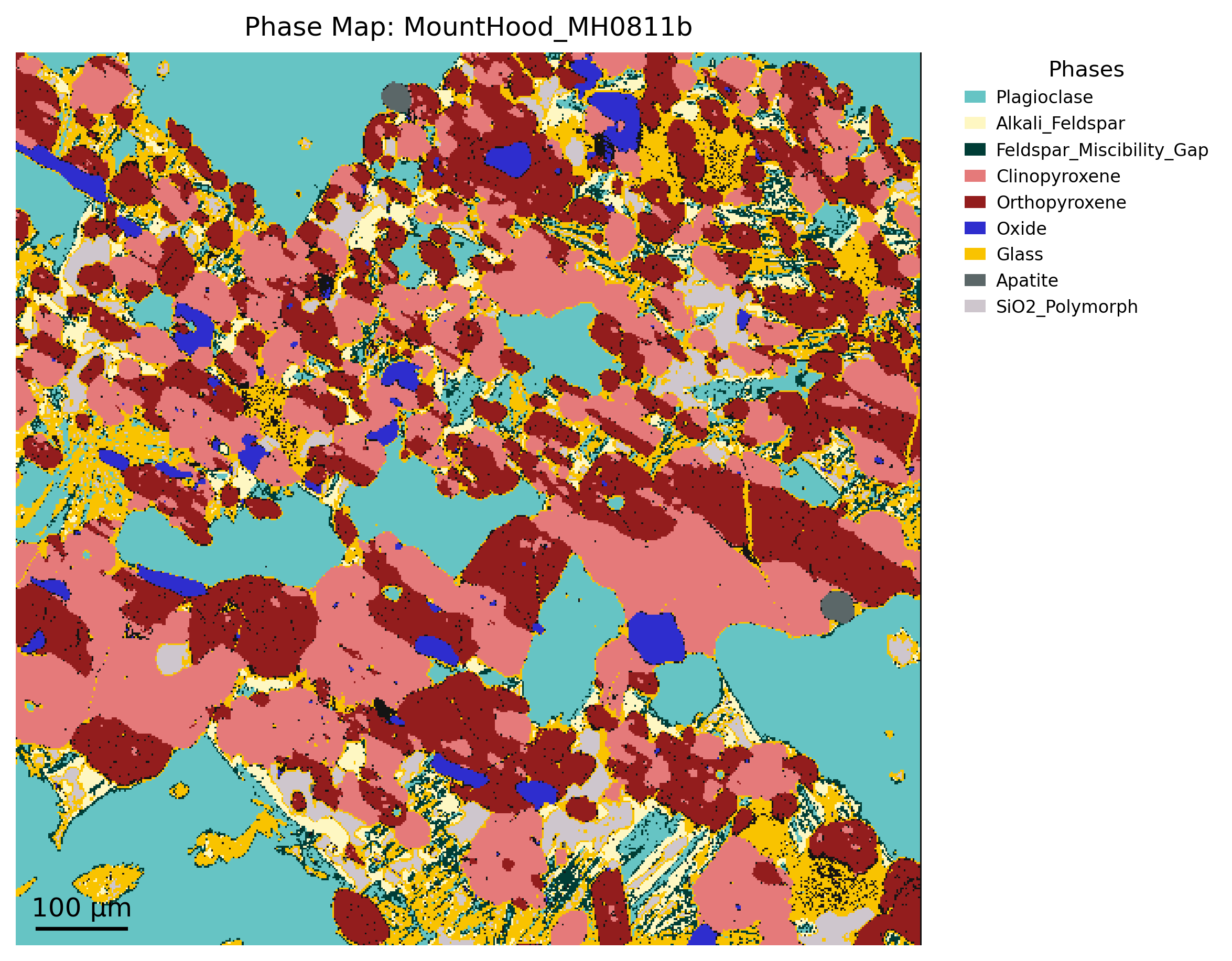
[12]:
# EDS phase map
output['figs'][0]
[12]:

We can now examine the phase maps produced by the two methods and compare their performance. See the preprint for a more detailed description of these maps.
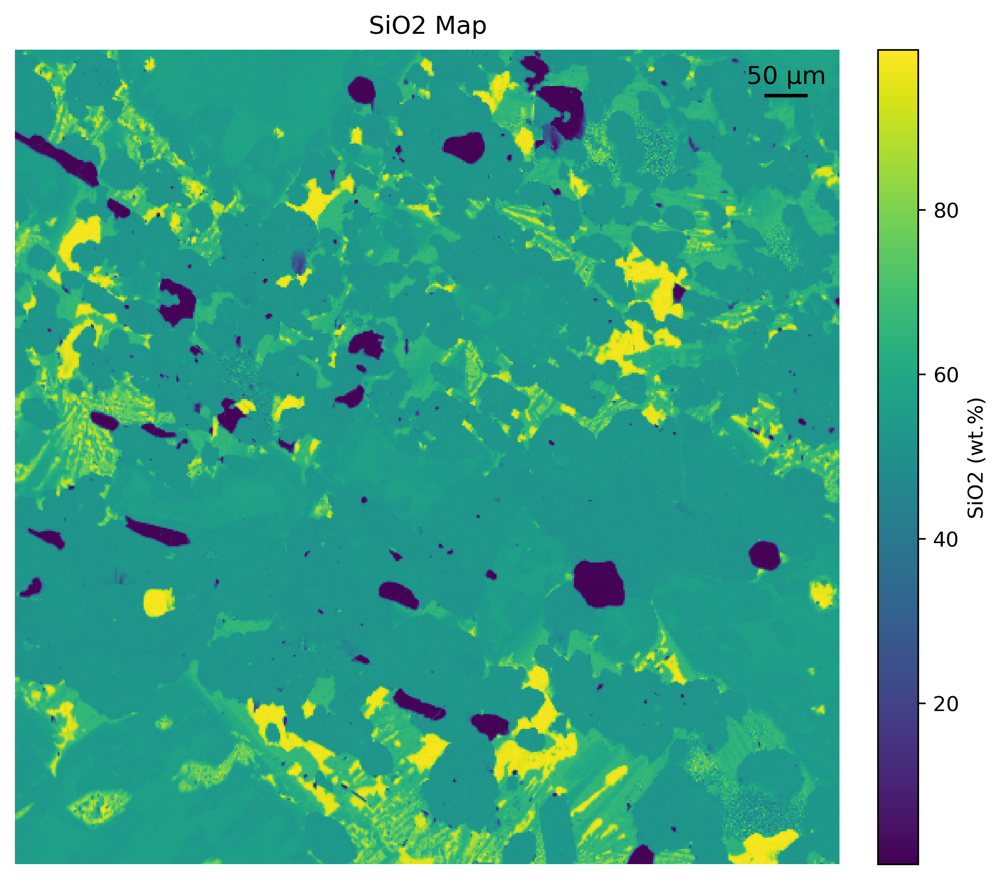
5. Plot oxide concentration maps and prediction score maps
Let’s plot the original oxide maps loaded from the directory. We can examine how well the predicted phase map matches some of the observations made in oxide space. We have a handy function for doing so, with mm.plot_oxide_map.
[13]:
fig, ax = mm.plot_oxide_map(
    output, # take the output from run_map
    oxide_name='SiO2', # specify the oxide of interest
    scalebar_um=50, # define size of scalebar desired, in microns
    pixel_size_um=2, # define size of each pixel of scalebar, in microns
    scalebar_loc='upper right', # specify location for scalebar
    scalebar_col='black', # specify color for scalebar
)
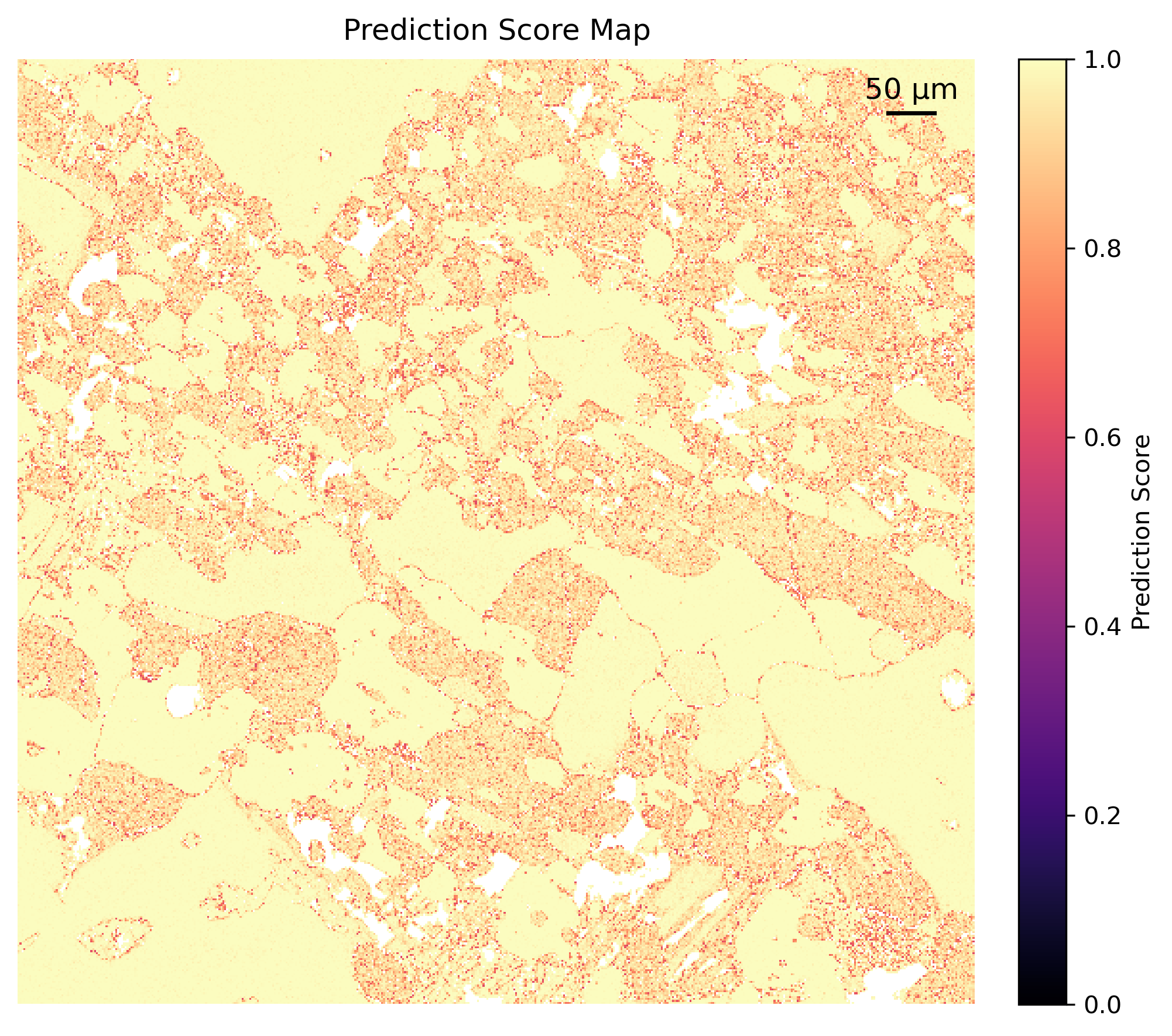
Let’s plot the prediction scores from the output, in mapped form. This allows for further investigation to determine where predictions are more and less certain.
[14]:
fig, ax = mm.plot_score_map(
    output, # take the output from run_map
    scalebar_um=50, # define size of scalebar desired, in microns
    pixel_size_um=2, # define size of each pixel of scalebar, in microns
    scalebar_loc='upper right', # specify location for scalebar
    scalebar_col='black', # specify color for scalebar
)
6. Plot compositions of mapped minerals in various classification diagrams (ternary, quadrilateral).
We can do some more with mineralML now. Let’s plot all the feldspars, pyroxenes, and spinels in ternary space.
Identify the phases present.
[15]:
# Here are all our feldspars
fspars = df_pred[df_pred.Predict_Mineral == 'Plagioclase']
display('Feldspars:', fspars)

# Here are all our pyroxenes
pxs_names = ['Clinopyroxene', 'Orthopyroxene']
pxs = df_pred[df_pred.Predict_Mineral.isin(pxs_names)]
display('Pyroxenes:', pxs)

# Here are all our oxides
ox_names = ['Oxide']
oxs = df_pred[df_pred.Predict_Mineral.isin(ox_names)]
display('Oxides:', oxs)
'Feldspars:'
| SiO2 | TiO2 | Al2O3 | FeOt | MnO | MgO | CaO | Na2O | K2O | Cr2O3 | P2O5 | ZrO2 | Predict_Mineral | Prediction_Score | Prediction_Score_Sigma | Second_Predict_Mineral | Second_Prediction_Score | Submineral | |
|---|---|---|---|---|---|---|---|---|---|---|---|---|---|---|---|---|---|---|
| 6 | 59.409736 | 0.453551 | 24.911057 | 0.437281 | 0.112236 | 0.207861 | 6.787231 | 6.732034 | 0.948753 | 0.000000 | 0.000000 | NaN | Plagioclase | 0.998052 | 0.010622 | Glass | 0.001846 | Andesine |
| 7 | 57.293535 | 0.000000 | 26.530507 | 1.352565 | 0.000000 | 0.388365 | 8.102746 | 5.804944 | 0.458178 | 0.000000 | 0.069160 | NaN | Plagioclase | 0.992805 | 0.040456 | Glass | 0.007124 | Andesine |
| 8 | 55.435543 | 0.033904 | 25.553034 | 1.356231 | 0.297159 | 0.040152 | 9.300065 | 5.570140 | 0.949996 | 0.595895 | 0.000000 | NaN | Plagioclase | 0.988094 | 0.025955 | Glass | 0.011509 | Andesine |
| 9 | 55.594348 | 0.000000 | 27.377475 | 1.390827 | 0.010037 | 0.019643 | 8.963531 | 5.725492 | 0.710503 | 0.208144 | 0.000000 | NaN | Plagioclase | 0.998130 | 0.007349 | Glass | 0.001659 | Andesine |
| 10 | 55.342296 | 0.031976 | 27.614579 | 1.644185 | 0.000000 | 0.082248 | 9.629535 | 5.026421 | 0.508073 | 0.000000 | 0.000000 | NaN | Plagioclase | 0.991868 | 0.049857 | Glass | 0.007949 | Andesine |
| ... | ... | ... | ... | ... | ... | ... | ... | ... | ... | ... | ... | ... | ... | ... | ... | ... | ... | ... |
| 247253 | 65.628218 | 0.102233 | 20.322669 | 0.970144 | 0.000000 | 0.225444 | 3.856563 | 6.940244 | 1.429413 | 0.525072 | 0.000000 | NaN | Plagioclase | 0.920885 | 0.178779 | Glass | 0.077788 | Oligoclase |
| 247260 | 64.632527 | 0.076708 | 21.037032 | 0.653223 | 0.000000 | 0.119711 | 3.751034 | 7.452901 | 1.592908 | 0.069690 | 0.000000 | NaN | Plagioclase | 0.987307 | 0.027464 | Glass | 0.011845 | Oligoclase |
| 247262 | 64.296102 | 0.000000 | 21.485038 | 0.976630 | 0.000000 | 0.233654 | 3.234296 | 7.440961 | 2.012244 | 0.293341 | 0.027735 | NaN | Plagioclase | 0.980832 | 0.088832 | Glass | 0.018718 | Oligoclase |
| 247288 | 60.975595 | 0.000000 | 22.110719 | 1.477735 | 0.102445 | 1.313905 | 5.829286 | 7.125921 | 1.005915 | 0.058480 | 0.000000 | NaN | Plagioclase | 0.967834 | 0.088990 | Glass | 0.031806 | Oligoclase |
| 247480 | 63.657836 | 0.455971 | 21.603974 | 1.279722 | 0.000000 | 0.323472 | 3.743229 | 7.084680 | 1.518178 | 0.270450 | 0.062488 | NaN | Plagioclase | 0.990895 | 0.026728 | Glass | 0.008367 | Oligoclase |
57198 rows × 18 columns
'Pyroxenes:'
| SiO2 | TiO2 | Al2O3 | FeOt | MnO | MgO | CaO | Na2O | K2O | Cr2O3 | P2O5 | ZrO2 | Predict_Mineral | Prediction_Score | Prediction_Score_Sigma | Second_Predict_Mineral | Second_Prediction_Score | Submineral | |
|---|---|---|---|---|---|---|---|---|---|---|---|---|---|---|---|---|---|---|
| 0 | 52.869693 | 0.089446 | 1.409243 | 21.357081 | 0.382089 | 21.732924 | 1.831746 | 0.069385 | 0.182859 | 0.000000 | 0.000000 | NaN | Orthopyroxene | 0.954259 | 0.121515 | Amphibole | 0.045181 | Enstatite |
| 1 | 51.892819 | 0.591858 | 1.289309 | 22.414176 | 1.120519 | 20.739631 | 1.453647 | 0.155577 | 0.000000 | 0.000000 | 0.000000 | NaN | Orthopyroxene | 0.926802 | 0.161589 | Amphibole | 0.072842 | Enstatite |
| 2 | 52.287424 | 0.306354 | 0.442857 | 22.273798 | 0.656842 | 21.441527 | 1.709473 | 0.313483 | 0.159156 | 0.326132 | 0.000000 | NaN | Orthopyroxene | 0.937167 | 0.156033 | Amphibole | 0.053794 | Enstatite |
| 3 | 51.667645 | 0.468977 | 1.602369 | 23.606152 | 0.000000 | 20.711076 | 1.316344 | 0.364752 | 0.000000 | 0.000000 | 0.000000 | NaN | Orthopyroxene | 0.868075 | 0.213352 | Amphibole | 0.130258 | Enstatite |
| 4 | 53.113961 | 0.000000 | 1.850691 | 22.954577 | 0.603992 | 19.687578 | 1.703375 | 0.000000 | 0.078555 | 0.007271 | 0.000000 | NaN | Orthopyroxene | 0.955211 | 0.083039 | Amphibole | 0.041217 | Enstatite |
| ... | ... | ... | ... | ... | ... | ... | ... | ... | ... | ... | ... | ... | ... | ... | ... | ... | ... | ... |
| 247471 | 52.777936 | 0.341422 | 0.681463 | 22.052613 | 0.492089 | 21.713396 | 1.409693 | 0.000000 | 0.014347 | 0.128819 | 0.388221 | NaN | Orthopyroxene | 0.924290 | 0.209623 | Amphibole | 0.071631 | Enstatite |
| 247472 | 51.164731 | 0.033477 | 0.757427 | 23.908463 | 1.223195 | 20.198822 | 1.584169 | 0.034482 | 0.115519 | 0.426862 | 0.000000 | NaN | Orthopyroxene | 0.963717 | 0.129811 | Amphibole | 0.035776 | Enstatite |
| 247490 | 52.781085 | 0.000000 | 1.084068 | 25.244632 | 0.585867 | 18.465076 | 1.386827 | 0.436795 | 0.000000 | 0.000000 | 0.015651 | NaN | Orthopyroxene | 0.800574 | 0.286466 | Amphibole | 0.195758 | Enstatite |
| 247491 | 52.136743 | 0.332666 | 0.759727 | 23.384690 | 0.000000 | 21.442475 | 1.262017 | 0.000000 | 0.000000 | 0.573398 | 0.000000 | NaN | Orthopyroxene | 0.955728 | 0.141057 | Amphibole | 0.043054 | Enstatite |
| 247492 | 52.276311 | 0.283907 | 1.219325 | 21.488206 | 0.775673 | 21.428622 | 1.410546 | 0.323923 | 0.107557 | 0.174155 | 0.000000 | NaN | Orthopyroxene | 0.762849 | 0.309576 | Amphibole | 0.236592 | Enstatite |
115035 rows × 18 columns
'Oxides:'
| SiO2 | TiO2 | Al2O3 | FeOt | MnO | MgO | CaO | Na2O | K2O | Cr2O3 | P2O5 | ZrO2 | Predict_Mineral | Prediction_Score | Prediction_Score_Sigma | Second_Predict_Mineral | Second_Prediction_Score | Submineral | |
|---|---|---|---|---|---|---|---|---|---|---|---|---|---|---|---|---|---|---|
| 816 | 9.601393 | 42.543327 | 0.726077 | 42.288306 | 0.000000 | 3.217761 | 1.174167 | 0.000000 | 0.234858 | 0.000000 | 0.047997 | NaN | Oxide | 0.991546 | 0.027993 | Olivine | 0.006062 | Rhombohedral_Oxides |
| 817 | 5.055912 | 45.136092 | 0.727534 | 46.073721 | 1.004736 | 1.408648 | 0.391981 | 0.057390 | 0.056051 | 0.047390 | 0.040546 | NaN | Oxide | 0.999652 | 0.000546 | Olivine | 0.000150 | Rhombohedral_Oxides |
| 1317 | 14.740859 | 37.393898 | 4.124402 | 38.457593 | 0.104994 | 2.263607 | 2.124805 | 0.105771 | 0.285457 | 0.398615 | 0.000000 | NaN | Oxide | 0.942460 | 0.152996 | Amphibole | 0.027525 | Rhombohedral_Oxides |
| 1318 | 5.418784 | 43.949746 | 3.063736 | 45.020854 | 0.556096 | 0.814851 | 0.223852 | 0.000000 | 0.101373 | 0.000000 | 0.000000 | NaN | Oxide | 0.997249 | 0.010152 | Chlorite | 0.001335 | Rhombohedral_Oxides |
| 1319 | 2.445324 | 47.957417 | 0.453160 | 46.692280 | 0.711513 | 0.676563 | 0.358138 | 0.221529 | 0.119474 | 0.151114 | 0.000000 | NaN | Oxide | 0.998311 | 0.008520 | Kalsilite | 0.000778 | Rhombohedral_Oxides |
| ... | ... | ... | ... | ... | ... | ... | ... | ... | ... | ... | ... | ... | ... | ... | ... | ... | ... | ... |
| 247375 | 1.709557 | 12.717564 | 1.237637 | 83.124692 | 0.166292 | 0.681558 | 0.092660 | 0.000000 | 0.000000 | 0.270039 | 0.000000 | NaN | Oxide | 0.999055 | 0.005121 | Olivine | 0.000901 | Spinel_Group |
| 247376 | 1.949185 | 11.587195 | 1.197346 | 82.621199 | 0.856195 | 0.850968 | 0.195952 | 0.000000 | 0.000000 | 0.384142 | 0.120489 | NaN | Oxide | 0.999924 | 0.000488 | Olivine | 0.000043 | Spinel_Group |
| 247377 | 0.929317 | 12.592958 | 1.076223 | 82.325128 | 0.033928 | 1.037305 | 0.338269 | 0.295170 | 0.298730 | 1.023496 | 0.000000 | NaN | Oxide | 0.999981 | 0.000345 | Epidote | 0.000011 | Spinel_Group |
| 247378 | 1.137157 | 12.901928 | 1.104496 | 82.801424 | 0.117042 | 1.164574 | 0.225610 | 0.000000 | 0.070023 | 0.212909 | 0.264837 | NaN | Oxide | 0.996252 | 0.026203 | Nepheline | 0.003743 | Spinel_Group |
| 247379 | 5.987311 | 11.661483 | 2.857898 | 76.584670 | 0.261887 | 0.624719 | 0.561372 | 0.730096 | 0.029141 | 0.701422 | 0.000000 | NaN | Oxide | 0.999971 | 0.000000 | Rhombohedral_Oxides | 0.000012 | Spinel_Group |
5568 rows × 18 columns
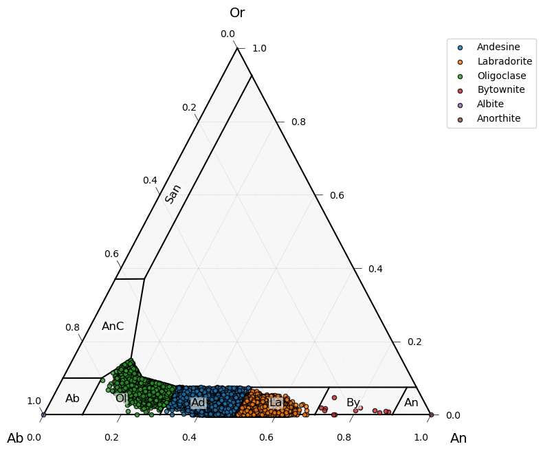
Plot these feldspars, pyroxenes, and spinels!
[16]:
# Use FeldsparClassifier to examine at the component space (XAn, XAb, XOr)
fspar_comp = mm.FeldsparClassifier(fspars).calculate_components()
display(fspar_comp)

# Use FeldsparClassifier to plot up these data.
fig = mm.FeldsparClassifier(fspars).plot()
| Sample | SiO2 | TiO2 | Al2O3 | FeOt | MnO | MgO | CaO | Na2O | K2O | ... | Prediction_Score | Prediction_Score_Sigma | Second_Predict_Mineral | Second_Prediction_Score | Cation_Sum | M_site | T_site | An | Ab | Or | |
|---|---|---|---|---|---|---|---|---|---|---|---|---|---|---|---|---|---|---|---|---|---|
| 6 | NaN | 59.409736 | 0.453551 | 24.911057 | 0.437281 | 0.112236 | 0.207861 | 6.787231 | 6.732034 | 0.948753 | ... | 0.998052 | 0.010622 | Glass | 0.001846 | 4.987375 | 0.963944 | 3.973663 | 0.337691 | 0.606105 | 0.056204 |
| 7 | NaN | 57.293535 | 0.000000 | 26.530507 | 1.352565 | 0.000000 | 0.388365 | 8.102746 | 5.804944 | 0.458178 | ... | 0.992805 | 0.040456 | Glass | 0.007124 | 4.983526 | 0.922530 | 3.981485 | 0.423060 | 0.548456 | 0.028483 |
| 8 | NaN | 55.435543 | 0.033904 | 25.553034 | 1.356231 | 0.297159 | 0.040152 | 9.300065 | 5.570140 | 0.949996 | ... | 0.988094 | 0.025955 | Glass | 0.011509 | 5.026741 | 1.009083 | 3.928468 | 0.453425 | 0.491428 | 0.055148 |
| 9 | NaN | 55.594348 | 0.000000 | 27.377475 | 1.390827 | 0.010037 | 0.019643 | 8.963531 | 5.725492 | 0.710503 | ... | 0.998130 | 0.007349 | Glass | 0.001659 | 5.019667 | 0.978708 | 3.979120 | 0.444396 | 0.513663 | 0.041941 |
| 10 | NaN | 55.342296 | 0.031976 | 27.614579 | 1.644185 | 0.000000 | 0.082248 | 9.629535 | 5.026421 | 0.508073 | ... | 0.991868 | 0.049857 | Glass | 0.007949 | 4.989487 | 0.938373 | 3.982168 | 0.498163 | 0.470542 | 0.031295 |
| ... | ... | ... | ... | ... | ... | ... | ... | ... | ... | ... | ... | ... | ... | ... | ... | ... | ... | ... | ... | ... | ... |
| 247253 | NaN | 65.628218 | 0.102233 | 20.322669 | 0.970144 | 0.000000 | 0.225444 | 3.856563 | 6.940244 | 1.429413 | ... | 0.920885 | 0.178779 | Glass | 0.077788 | 4.892980 | 0.858505 | 3.961967 | 0.212866 | 0.693194 | 0.093940 |
| 247260 | NaN | 64.632527 | 0.076708 | 21.037032 | 0.653223 | 0.000000 | 0.119711 | 3.751034 | 7.452901 | 1.592908 | ... | 0.987307 | 0.027464 | Glass | 0.011845 | 4.932751 | 0.912954 | 3.982498 | 0.196039 | 0.704840 | 0.099121 |
| 247262 | NaN | 64.296102 | 0.000000 | 21.485038 | 0.976630 | 0.000000 | 0.233654 | 3.234296 | 7.440961 | 2.012244 | ... | 0.980832 | 0.088832 | Glass | 0.018718 | 4.952414 | 0.908712 | 3.980610 | 0.169378 | 0.705150 | 0.125471 |
| 247288 | NaN | 60.975595 | 0.000000 | 22.110719 | 1.477735 | 0.102445 | 1.313905 | 5.829286 | 7.125921 | 1.005915 | ... | 0.967834 | 0.088990 | Glass | 0.031806 | 5.015272 | 0.958287 | 3.907595 | 0.292609 | 0.647272 | 0.060120 |
| 247480 | NaN | 63.657836 | 0.455971 | 21.603974 | 1.279722 | 0.000000 | 0.323472 | 3.743229 | 7.084680 | 1.518178 | ... | 0.990895 | 0.026728 | Glass | 0.008367 | 4.930467 | 0.874556 | 3.959842 | 0.203757 | 0.697848 | 0.098395 |
57198 rows × 58 columns
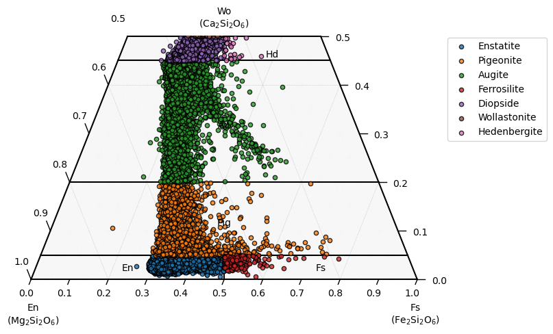
[17]:
# Use PyroxeneClassifier to examine at the component space (En, Wo, Fs). If sodic pyroxenes are also within this input, this will plot them up in the sodic pyroxene ternary
pxs_comp = mm.PyroxeneClassifier(pxs).calculate_components()
display(pxs_comp)

# Use PyroxeneClassifier to plot up these data.
fig = mm.PyroxeneClassifier(pxs).plot()
| Sample | SiO2 | TiO2 | Al2O3 | FeOt | MnO | MgO | CaO | Na2O | K2O | ... | EnFs | DiHd_2003 | Di | Fe3_Wang21 | Fe2_Wang21 | Di_h | Hd_h | Aeg_h | Jd_h | En_h | |
|---|---|---|---|---|---|---|---|---|---|---|---|---|---|---|---|---|---|---|---|---|---|
| 0 | NaN | 52.869693 | 0.089446 | 1.409243 | 21.357081 | 0.382089 | 21.732924 | 1.831746 | 0.069385 | 0.182859 | ... | 0.913586 | 0.044671 | 0.028612 | -0.000221 | 0.665433 | 0.042671 | 0.0 | 0.008467 | 0.002725 | 0.914269 |
| 1 | NaN | 51.892819 | 0.591858 | 1.289309 | 22.414176 | 1.120519 | 20.739631 | 1.453647 | 0.155577 | 0.000000 | ... | 0.917508 | 0.035731 | 0.021827 | 0.010831 | 0.695281 | 0.027619 | 0.0 | 0.000000 | 0.000000 | 0.931327 |
| 2 | NaN | 52.287424 | 0.306354 | 0.442857 | 22.273798 | 0.656842 | 21.441527 | 1.709473 | 0.313483 | 0.159156 | ... | 0.927521 | 0.046937 | 0.029333 | 0.029976 | 0.670329 | 0.023331 | 0.0 | 0.012125 | 0.000000 | 0.910934 |
| 3 | NaN | 51.667645 | 0.468977 | 1.602369 | 23.606152 | 0.000000 | 20.711076 | 1.316344 | 0.364752 | 0.000000 | ... | 0.940243 | 0.026458 | 0.016139 | 0.035618 | 0.708142 | 0.004287 | 0.0 | 0.013351 | 0.000000 | 0.924734 |
| 4 | NaN | 53.113961 | 0.000000 | 1.850691 | 22.954577 | 0.603992 | 19.687578 | 1.703375 | 0.000000 | 0.078555 | ... | 0.907582 | 0.000240 | 0.000144 | -0.054452 | 0.772333 | 0.029232 | 0.0 | 0.000000 | 0.003748 | 0.902651 |
| ... | ... | ... | ... | ... | ... | ... | ... | ... | ... | ... | ... | ... | ... | ... | ... | ... | ... | ... | ... | ... | ... |
| 247471 | NaN | 52.777936 | 0.341422 | 0.681463 | 22.052613 | 0.492089 | 21.713396 | 1.409693 | 0.000000 | 0.014347 | ... | 0.927852 | 0.037868 | 0.023927 | 0.010103 | 0.677190 | 0.032816 | 0.0 | 0.000000 | 0.000000 | 0.938144 |
| 247472 | NaN | 51.164731 | 0.033477 | 0.757427 | 23.908463 | 1.223195 | 20.198822 | 1.584169 | 0.034482 | 0.115519 | ... | 0.938871 | 0.034974 | 0.020592 | 0.034501 | 0.728767 | 0.000000 | 0.0 | 0.000000 | 0.000000 | 0.936789 |
| 247490 | NaN | 52.781085 | 0.000000 | 1.084068 | 25.244632 | 0.585867 | 18.465076 | 1.386827 | 0.436795 | 0.000000 | ... | 0.898961 | 0.042573 | 0.023851 | -0.011006 | 0.809892 | 0.048076 | 0.0 | 0.000000 | 0.032046 | 0.905598 |
| 247491 | NaN | 52.136743 | 0.332666 | 0.759727 | 23.384690 | 0.000000 | 21.442475 | 1.262017 | 0.000000 | 0.000000 | ... | 0.957045 | 0.021888 | 0.013580 | 0.004964 | 0.729895 | 0.012807 | 0.0 | 0.000000 | 0.000000 | 0.952504 |
| 247492 | NaN | 52.276311 | 0.283907 | 1.219325 | 21.488206 | 0.775673 | 21.428622 | 1.410546 | 0.323923 | 0.107557 | ... | 0.919233 | 0.035533 | 0.022445 | 0.022909 | 0.651775 | 0.020572 | 0.0 | 0.015542 | 0.000000 | 0.918074 |
115035 rows × 86 columns
/home/docs/checkouts/readthedocs.org/user_builds/mineralml/conda/stable/lib/python3.9/site-packages/ternary/plotting.py:148: UserWarning: No data for colormapping provided via 'c'. Parameters 'vmin', 'vmax' will be ignored
  ax.scatter(xs, ys, vmin=vmin, vmax=vmax, **kwargs)
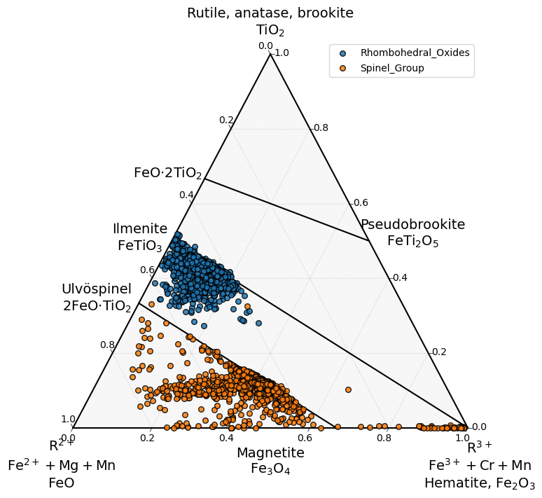
[18]:
# Use OxideClassifier to examine at the component space.
oxs_comp = mm.OxideClassifier(oxs).calculate_components()
display(oxs_comp)

# Use OxideClassifier to plot up these data.
fig = mm.OxideClassifier(oxs).plot()
| SiO2 | TiO2 | Al2O3 | FeOt | MnO | MgO | CaO | Na2O | K2O | Cr2O3 | ... | Fe2t_cat_4ox | Fe2_cat_4ox | Fe3_cat_4ox | Mn_cat_4ox | Mg_cat_4ox | Ca_cat_4ox | Na_cat_4ox | K_cat_4ox | P_cat_4ox | Cr_cat_4ox | |
|---|---|---|---|---|---|---|---|---|---|---|---|---|---|---|---|---|---|---|---|---|---|
| 816 | 9.601393 | 42.543327 | 0.726077 | 42.288306 | 0.000000 | 3.217761 | 1.174167 | 0.000000 | 0.234858 | 0.000000 | ... | NaN | NaN | NaN | NaN | NaN | NaN | NaN | NaN | NaN | NaN |
| 817 | 5.055912 | 45.136092 | 0.727534 | 46.073721 | 1.004736 | 1.408648 | 0.391981 | 0.057390 | 0.056051 | 0.047390 | ... | NaN | NaN | NaN | NaN | NaN | NaN | NaN | NaN | NaN | NaN |
| 1317 | 14.740859 | 37.393898 | 4.124402 | 38.457593 | 0.104994 | 2.263607 | 2.124805 | 0.105771 | 0.285457 | 0.398615 | ... | NaN | NaN | NaN | NaN | NaN | NaN | NaN | NaN | NaN | NaN |
| 1318 | 5.418784 | 43.949746 | 3.063736 | 45.020854 | 0.556096 | 0.814851 | 0.223852 | 0.000000 | 0.101373 | 0.000000 | ... | NaN | NaN | NaN | NaN | NaN | NaN | NaN | NaN | NaN | NaN |
| 1319 | 2.445324 | 47.957417 | 0.453160 | 46.692280 | 0.711513 | 0.676563 | 0.358138 | 0.221529 | 0.119474 | 0.151114 | ... | NaN | NaN | NaN | NaN | NaN | NaN | NaN | NaN | NaN | NaN |
| ... | ... | ... | ... | ... | ... | ... | ... | ... | ... | ... | ... | ... | ... | ... | ... | ... | ... | ... | ... | ... | ... |
| 247375 | 1.709557 | 12.717564 | 1.237637 | 83.124692 | 0.166292 | 0.681558 | 0.092660 | 0.000000 | 0.000000 | 0.270039 | ... | 2.490985 | 1.359076 | 1.131909 | 0.005047 | 0.036407 | 0.003557 | 0.000000 | 0.000000 | 0.000000 | 0.007650 |
| 247376 | 1.949185 | 11.587195 | 1.197346 | 82.621199 | 0.856195 | 0.850968 | 0.195952 | 0.000000 | 0.000000 | 0.384142 | ... | 2.474110 | 1.310324 | 1.163786 | 0.025967 | 0.045423 | 0.007518 | 0.000000 | 0.000000 | 0.003652 | 0.010875 |
| 247377 | 0.929317 | 12.592958 | 1.076223 | 82.325128 | 0.033928 | 1.037305 | 0.338269 | 0.295170 | 0.298730 | 1.023496 | ... | 2.452451 | 1.233630 | 1.218821 | 0.001024 | 0.055082 | 0.012910 | 0.020385 | 0.013575 | 0.000000 | 0.028824 |
| 247378 | 1.137157 | 12.901928 | 1.104496 | 82.801424 | 0.117042 | 1.164574 | 0.225610 | 0.000000 | 0.070023 | 0.212909 | ... | 2.474554 | 1.322909 | 1.151645 | 0.003543 | 0.062039 | 0.008638 | 0.000000 | 0.003192 | 0.008012 | 0.006015 |
| 247379 | 5.987311 | 11.661483 | 2.857898 | 76.584670 | 0.261887 | 0.624719 | 0.561372 | 0.730096 | 0.029141 | 0.701422 | ... | 2.235827 | 1.352598 | 0.883229 | 0.007743 | 0.032510 | 0.020997 | 0.049414 | 0.001298 | 0.000000 | 0.019359 |
5568 rows × 92 columns
/home/docs/checkouts/readthedocs.org/user_builds/mineralml/conda/stable/lib/python3.9/site-packages/ternary/plotting.py:148: UserWarning: No data for colormapping provided via 'c'. Parameters 'vmin', 'vmax' will be ignored
  ax.scatter(xs, ys, vmin=vmin, vmax=vmax, **kwargs)
/home/docs/checkouts/readthedocs.org/user_builds/mineralml/conda/stable/lib/python3.9/site-packages/ternary/plotting.py:148: UserWarning: No data for colormapping provided via 'c'. Parameters 'vmin', 'vmax' will be ignored
  ax.scatter(xs, ys, vmin=vmin, vmax=vmax, **kwargs)
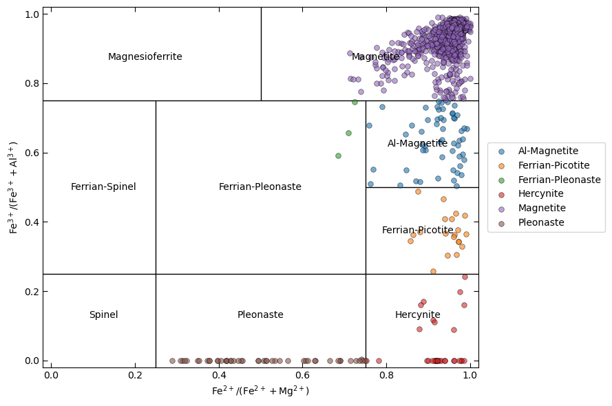
You might note that the structure of these three ...Classifier classes is identical. That is intentional! mm.FeldsparClassifier, mm.PyroxeneClassifier, and mm.OxideClassifier all have calculate_components and plot methods embedded.
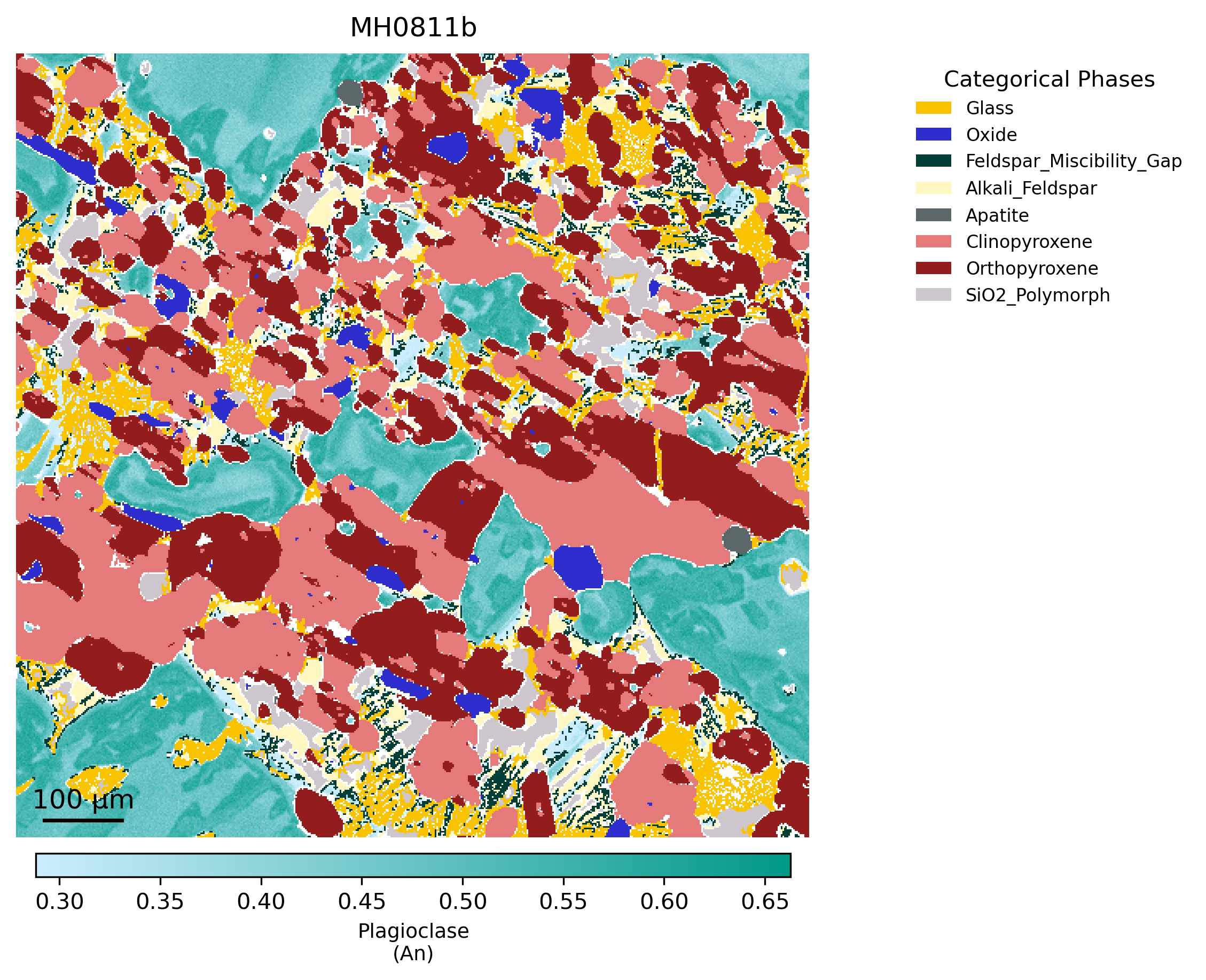
7. Plot chemical variation maps
We know the mineralogy now. What if you now want to inspect the chemical variation within the individual crystals? Pull the component maps created for each sample and plot this up with mm.plot_component_composite.
This function currently does this calculation for feldspars, pyroxenes, olivines, and amphibole. This can easily be expanded with all the stoichiometric mineral functions. Here, I will just show this for these common igneous phases.
[19]:
# Inspect what’s available:
print(sorted(output["component_maps"].keys()))

#  Plot map highlighting internal compositional variation
fig = mm.plot_component_composite(output, # specify output from above
                                  title="MH0811b", # optionally add a title to this plot
                                  phases=mh_base_cols.keys(), # phases of interest
                                  phase_colors=mh_base_cols, # provide a color scheme for the phases, as a dictionary mapping phase names to color codes
                                  smooth_sigma=0.25, # add a Gaussian blur to smooth compositional data, usually turned off.
                                  scalebar_um=100, # define size of scalebar desired, in microns
                                  pixel_size_um=2.0, # define size of each pixel of scalebar, in microns
                                  scalebar_loc='lower left', # specify location for scalebar
                                  scalebar_col='black', # specify color for scalebar
                                  )
['Clinopyroxene.En', 'Clinopyroxene.Fs', 'Clinopyroxene.Wo', 'Feldspar.Ab', 'Feldspar.An', 'Feldspar.Or', 'Orthopyroxene.En', 'Orthopyroxene.Fs', 'Orthopyroxene.Wo']
One could alternatively use all the functions within mineralML.mapping to do these same things, in a more stepwise manner. Look through the documentation if you would like to use individual bits of this code.