This page was generated from
docs/examples/mineralML_microanalysisoutput.ipynb.
Interactive online version:
![]() .
.
[1]:
""" Created on March 26, 2026 // @author: Sarah Shi """

import os
import numpy as np
import pandas as pd

import mineralML as mm
import Thermobar as pt

import matplotlib.pyplot as plt
%matplotlib inline
%config InlineBackend.figure_format = 'png'
mineralML Quickstart for Tabular Microanalytical Data
This notebook shows how to load and run your microanalytical data through mineralML, across a number of different formats returned straight from Cameca, Probe for EPMA, and AZtec (Oxford Instruments). This is a five step process:
Extract and standardize data from raw instrument files (Excel or CSV) using
mm.extract_cameca,mm.extract_probe4epma, ormm.extract_aztec. For reference, the common outputs for these three types of instruments is provided on GitHub (https://github.com/sarahshi/mineralML/tree/main/docs/TabularData/microanalysis.xlsx), in the three sheets. Clean and align columns withmm.prep_df.Run data through the neural network with
mm.predict_class_probto derive classifications and prediction scores.Export predictions and prediction scores with
mm.export_predictions_to_excel.Calculate mineral compositions and plot compositions in empirical classification space (ternaries, quadrilaterals).
Run data through
Thermobarfor thermobarometric estimates.
We loaded in the mineralML Python package as mm. mineralML has trained machine learning models for classifying minerals. This implementation aims to get your electron microprobe or quantitative EDS compositions classified and processed. We remove some degrees of freedom to simplify the process as much as possible. The minerals considered for this study include: Amphibole, Apatite, Biotite, Calcite, Chlorite, Epidote, Feldspar (Alkali Feldspar and Plagioclase), Garnet, Glass,
Kalsilite, Leucite, Melilite, Muscovite, Nepheline, Olivine, Oxide (Rhombohedral_Oxides including Hematite-Ilmenite, Spinel_Group including Magnetite-Spinel), Pyroxene (Clinopyroxene, Orthopyroxene, Na-Pyroxene), Quartz, Rutile, Serpentine, Titanite, Tourmaline, and Zircon.
An Excel or CSV file containing your electron microprobe or EDS analyses is necessary. Thanks to the integrated extraction functions, you no longer need to manually format complex headers or convert relative errors! Just point the correct extractor to your raw instrument export. The necessary oxides are SiO\(_2\), TiO\(_2\), Al\(_2\)O\(_3\), FeO\(_t\), MnO, MgO, CaO, Na\(_2\)O, K\(_2\)O, Cr\(_2\)O\(_3\), P\(_2\)O\(_5\), and ZrO\(_2\) (if you are aiming to classify zircon). For the oxides not analyzed for specific minerals, the preprocessing will fill in the nan values as 0.
We will apply the neural network method to the dataset.
1. Load and prepare data for analysis
We will use mm.extract_cameca, mm.extract_probe4epma, and mm.extract_aztec to extract the tabular data from their respective sheets in our EPMA dataset. Because these functions standardize the output format, we can easily combine them into a single dataframe before running them through mm.prep_df.
Note that the uncertainties from Cameca EPMAs are provided as 3 sigma! We convert these to 1 sigma.
[2]:
# Define the path to your microanalysis data output. Here, I've written three functions for dealing with Cameca, Probe for EPMA, and AZtec data outputs. If you have other outputs you'd like to work with, reach out and I can expand the functions available.
file_path = 'TabularData/microanalysis.xlsx'

# Extract data from each respective sheet/instrument
df_cameca = mm.extract_cameca(file_path, sheet_name='Cameca')
display('Cameca:', df_cameca.head())

df_p4e = mm.extract_probe4epma(file_path, sheet_name='Probe4EPMA')
display('Probe for EPMA:', df_p4e.head())

df_aztec = mm.extract_aztec(file_path, sheet_name='AZtec')
display('AZtec:', df_aztec.head())
'Cameca:'
| Sample | SiO2 | TiO2 | Al2O3 | FeOt | MnO | MgO | CaO | Na2O | K2O | ... | FeOt_1sigma | MnO_1sigma | MgO_1sigma | CaO_1sigma | Na2O_1sigma | K2O_1sigma | Cr2O3_1sigma | P2O5_1sigma | NiO_1sigma | O_1sigma | |
|---|---|---|---|---|---|---|---|---|---|---|---|---|---|---|---|---|---|---|---|---|---|
| 0 | Museum_Ol174.1_highcount_2 | 41.77717 | 0.000017 | 0.005657 | 9.425813 | 0.161341 | 49.51706 | 0.017556 | 0.000013 | 0.005696 | ... | 0.077547 | 0.011184 | 0.117512 | 0.006948 | -0.000116 | 0.004680 | -0.000028 | 0.003343 | 0.015145 | NaN |
| 1 | Museum_Ol174.1_highcount_2 | 41.71127 | 0.000017 | 0.000019 | 9.353550 | 0.121697 | 49.56913 | 0.034175 | 0.003019 | 0.008749 | ... | 0.077328 | 0.011659 | 0.117604 | 0.007157 | 0.004444 | 0.004610 | 0.009179 | 0.003529 | 0.015307 | NaN |
| 2 | Museum_Ol174.1_highcount_2 | 41.74872 | 0.000017 | 0.000019 | 9.297508 | 0.144290 | 49.75990 | 0.011651 | 0.000013 | 0.005699 | ... | 0.076868 | 0.011469 | 0.117930 | 0.006938 | -0.000015 | 0.004808 | -0.000013 | 0.003526 | 0.015003 | NaN |
| 3 | Museum_Ol174.1_highcount_2 | 41.87691 | 0.000017 | 0.000019 | 9.372102 | 0.116922 | 49.71903 | 0.023644 | 0.000013 | 0.000012 | ... | 0.077188 | 0.012172 | 0.117876 | 0.006977 | -0.000011 | -0.000011 | 0.009358 | 0.003245 | 0.015251 | NaN |
| 4 | Museum_Ol174.1_highcount_2 | 41.78258 | 0.000017 | 0.003852 | 9.354717 | 0.141731 | 49.81131 | 0.021923 | 0.001326 | 0.003255 | ... | 0.076843 | 0.011027 | 0.118055 | 0.006793 | 0.003950 | 0.004752 | 0.009304 | -0.000064 | 0.015466 | NaN |
5 rows × 27 columns
'Probe for EPMA:'
| Sample | SiO2 | TiO2 | Al2O3 | FeOt | MnO | MgO | CaO | Na2O | Cr2O3 | ... | SiO2_1sigma | TiO2_1sigma | Al2O3_1sigma | FeOt_1sigma | MnO_1sigma | MgO_1sigma | CaO_1sigma | Na2O_1sigma | Cr2O3_1sigma | NiO_1sigma | |
|---|---|---|---|---|---|---|---|---|---|---|---|---|---|---|---|---|---|---|---|---|---|
| 0 | TwinLakesDiopside | 56.7804 | 0.0 | 0.0 | 0.060834 | 0.000698 | 18.4330 | 25.7335 | 0.0 | 0.000000 | ... | 0.076460 | 0.0 | 0.0 | 0.006379 | 0.003544 | 0.027146 | 0.017425 | 0.0 | 0.000000 | 0.000000 |
| 1 | TwinLakesDiopside | 56.7965 | 0.0 | 0.0 | 0.062401 | 0.007511 | 18.4492 | 25.7467 | 0.0 | 0.000000 | ... | 0.076478 | 0.0 | 0.0 | 0.006488 | 0.003478 | 0.027160 | 0.017426 | 0.0 | 0.000000 | 0.003127 |
| 2 | TwinLakesDiopside | 56.6400 | 0.0 | 0.0 | 0.069621 | 0.004826 | 18.4928 | 25.7743 | 0.0 | 0.000000 | ... | 0.076339 | 0.0 | 0.0 | 0.006467 | 0.003484 | 0.027192 | 0.017432 | 0.0 | 0.000000 | 0.003112 |
| 3 | TwinLakesDiopside | 56.7002 | 0.0 | 0.0 | 0.055659 | 0.008368 | 18.4510 | 25.7420 | 0.0 | 0.002227 | ... | 0.076366 | 0.0 | 0.0 | 0.006336 | 0.003447 | 0.027157 | 0.017423 | 0.0 | 0.003274 | 0.000000 |
| 4 | TwinLakesDiopside | 56.7272 | 0.0 | 0.0 | 0.059733 | 0.001823 | 18.4430 | 25.7682 | 0.0 | 0.003180 | ... | 0.076406 | 0.0 | 0.0 | 0.006341 | 0.003463 | 0.027151 | 0.017429 | 0.0 | 0.003251 | 0.000000 |
5 rows × 22 columns
'AZtec:'
| Sample | SiO2 | TiO2 | Al2O3 | FeOt | MnO | MgO | CaO | Na2O | K2O | ... | Al2O3_1sigma | FeOt_1sigma | MnO_1sigma | MgO_1sigma | CaO_1sigma | Na2O_1sigma | K2O_1sigma | Cr2O3_1sigma | SO3_1sigma | NiO_1sigma | |
|---|---|---|---|---|---|---|---|---|---|---|---|---|---|---|---|---|---|---|---|---|---|
| 0 | Basalt_113716-1_1_WDS | 51.5531 | 1.3431 | 15.0794 | 9.2081 | 0.1651 | 8.0553 | 11.0920 | 2.7395 | 0.0719 | ... | 0.0368 | 0.0367 | 0.0154 | 0.0287 | 0.0267 | 0.0227 | 0.0086 | NaN | 0.0060 | NaN |
| 1 | Basalt_113716-1_2_WDS | 51.5500 | 1.3190 | 15.0192 | 9.1835 | 0.1710 | 8.0690 | 11.0471 | 2.7411 | 0.0699 | ... | 0.0368 | 0.0367 | 0.0154 | 0.0287 | 0.0267 | 0.0227 | 0.0087 | NaN | 0.0060 | NaN |
| 2 | Basalt_113716-1_3_WDS | 51.6652 | 1.3438 | 15.0686 | 9.2527 | 0.1555 | 8.0666 | 11.0889 | 2.7479 | 0.0775 | ... | 0.0368 | 0.0368 | 0.0154 | 0.0287 | 0.0267 | 0.0227 | 0.0086 | NaN | 0.0059 | NaN |
| 3 | Basalt_113716-1_4_WDS | 51.6838 | 1.3415 | 15.0678 | 9.2828 | 0.2064 | 8.0310 | 11.0918 | 2.7521 | 0.0809 | ... | 0.0368 | 0.0368 | 0.0154 | 0.0287 | 0.0267 | 0.0227 | 0.0086 | NaN | 0.0059 | NaN |
| 4 | Basalt_113716-1_5_WDS | 51.6122 | 1.3448 | 15.0311 | 9.1791 | 0.1597 | 8.0274 | 11.0576 | 2.7345 | 0.0740 | ... | 0.0367 | 0.0368 | 0.0154 | 0.0286 | 0.0267 | 0.0227 | 0.0086 | NaN | 0.0060 | NaN |
5 rows × 27 columns
[3]:
# Combine them into a single standardized dataframe
df_load = pd.concat([df_cameca, df_p4e, df_aztec], ignore_index=True)

# Prepare the dataframe by removing rows with too many NaNs, and filling in zeros.
df_nn = mm.prep_df(df_load, # dataframe to prepare
                   renormalize=False, # optionally renormalize rows to sum to 100 wt%
                   convert_fe=False, # optionally convert disparate input formats of Fe all to FeOt
                   drop_empty_rows=False, # optionally drop rows with more nan values than the min_oxide_count
                   min_oxide_count=2, # minimum number of oxides in a row to keep that analysis
                   verbose=True
                   )

# Examine the prepared dataframe
display(df_nn.head())
prep_df: 40 row(s) processed (of 40 input, 0 dropped).
/tmp/ipykernel_3320/1850373241.py:5: UserWarning: The following columns were missing and have been filled with NaN: ['ZrO2', 'Mineral']
  df_nn = mm.prep_df(df_load, # dataframe to prepare
| Sample | SiO2 | TiO2 | Al2O3 | FeOt | MnO | MgO | CaO | Na2O | K2O | ... | Na2O_1sigma | K2O_1sigma | Cr2O3_1sigma | P2O5_1sigma | NiO_1sigma | O_1sigma | O | SO3 | SO3_1sigma | Mineral | |
|---|---|---|---|---|---|---|---|---|---|---|---|---|---|---|---|---|---|---|---|---|---|
| 0 | Museum_Ol174.1_highcount_2 | 41.77717 | 0.000017 | 0.005657 | 9.425813 | 0.161341 | 49.51706 | 0.017556 | 0.000013 | 0.005696 | ... | -0.000116 | 0.004680 | -0.000028 | 0.003343 | 0.015145 | NaN | NaN | NaN | NaN | NaN |
| 1 | Museum_Ol174.1_highcount_2 | 41.71127 | 0.000017 | 0.000019 | 9.353550 | 0.121697 | 49.56913 | 0.034175 | 0.003019 | 0.008749 | ... | 0.004444 | 0.004610 | 0.009179 | 0.003529 | 0.015307 | NaN | NaN | NaN | NaN | NaN |
| 2 | Museum_Ol174.1_highcount_2 | 41.74872 | 0.000017 | 0.000019 | 9.297508 | 0.144290 | 49.75990 | 0.011651 | 0.000013 | 0.005699 | ... | -0.000015 | 0.004808 | -0.000013 | 0.003526 | 0.015003 | NaN | NaN | NaN | NaN | NaN |
| 3 | Museum_Ol174.1_highcount_2 | 41.87691 | 0.000017 | 0.000019 | 9.372102 | 0.116922 | 49.71903 | 0.023644 | 0.000013 | 0.000012 | ... | -0.000011 | -0.000011 | 0.009358 | 0.003245 | 0.015251 | NaN | NaN | NaN | NaN | NaN |
| 4 | Museum_Ol174.1_highcount_2 | 41.78258 | 0.000017 | 0.003852 | 9.354717 | 0.141731 | 49.81131 | 0.021923 | 0.001326 | 0.003255 | ... | 0.003950 | 0.004752 | 0.009304 | -0.000064 | 0.015466 | NaN | NaN | NaN | NaN | NaN |
5 rows × 32 columns
2. Apply the trained neural network (mm.predict_class_prob)
We will use mm.predict_class_prob to do so.
[4]:
# The trained neural network can be applied in just one line. It returns predictions in columns called "Predict_Mineral", "Submineral" (if applicable, for pyroxenes, feldspars, and oxides), "Predict_Probability", "Second_Predict_Mineral", "Second_Predict_Probability".

df_pred_nn = mm.predict_class_prob(df_nn)
mineralML: 40 rows — 40 classified by neural network, 0 by empirical rules (Zircon: 0, SiO2 polymorph: 0, Carbonate: 0), 0 skipped (invalid/empty)
[5]:
# Examine the predicted mineral classifications

display(df_pred_nn.head())
| Sample | SiO2 | TiO2 | Al2O3 | FeOt | MnO | MgO | CaO | Na2O | K2O | Cr2O3 | P2O5 | ZrO2 | Mineral | Predict_Mineral | Prediction_Score | Prediction_Score_Sigma | Second_Predict_Mineral | Second_Prediction_Score | Submineral | |
|---|---|---|---|---|---|---|---|---|---|---|---|---|---|---|---|---|---|---|---|---|
| 0 | Museum_Ol174.1_highcount_2 | 41.77717 | 0.000017 | 0.005657 | 9.425813 | 0.161341 | 49.51706 | 0.017556 | 0.000013 | 0.005696 | 0.000015 | 0.005393 | 0.0 | NaN | Olivine | 0.996502 | 0.052845 | Nepheline | 0.003324 | NaN |
| 1 | Museum_Ol174.1_highcount_2 | 41.71127 | 0.000017 | 0.000019 | 9.353550 | 0.121697 | 49.56913 | 0.034175 | 0.003019 | 0.008749 | 0.009664 | 0.001659 | 0.0 | NaN | Olivine | 0.999182 | 0.007934 | Serpentine | 0.000765 | NaN |
| 2 | Museum_Ol174.1_highcount_2 | 41.74872 | 0.000017 | 0.000019 | 9.297508 | 0.144290 | 49.75990 | 0.011651 | 0.000013 | 0.005699 | 0.000015 | 0.001245 | 0.0 | NaN | Olivine | 0.999268 | 0.007990 | Serpentine | 0.000495 | NaN |
| 3 | Museum_Ol174.1_highcount_2 | 41.87691 | 0.000017 | 0.000019 | 9.372102 | 0.116922 | 49.71903 | 0.023644 | 0.000013 | 0.000012 | 0.016916 | 0.002075 | 0.0 | NaN | Olivine | 0.992237 | 0.072574 | Apatite | 0.004258 | NaN |
| 4 | Museum_Ol174.1_highcount_2 | 41.78258 | 0.000017 | 0.003852 | 9.354717 | 0.141731 | 49.81131 | 0.021923 | 0.001326 | 0.003255 | 0.022817 | 0.000023 | 0.0 | NaN | Olivine | 0.999661 | 0.003711 | Serpentine | 0.000211 | NaN |
There is a good amount of information in this dataframe. The predicted mineral is provided in the Predict_Mineral column, along with the prediction score expressed in the Prediction_Score column (representing likelihood of prediction) and standard deviation on this prediction in the Prediction_Score_Sigma column.
[6]:
# Examine the unique predicted minerals.

print(np.unique(df_pred_nn.Predict_Mineral))
['Clinopyroxene' 'Glass' 'Olivine' 'Plagioclase']
3. Export prediction results
Say you would like to go back to working with Excel now. Use mm.export_predictions_to_excel to export the predictions and these values. All the original input data are returned in the first sheet, and data are split into individual mineral phases in all other sheets.
[7]:
# Export prediction results to an Excel workbook with one sheet called "All" containing all rows, and additional sheets for each predicted mineral.

mm.export_predictions_to_excel(df_pred_nn, filename='TabularData/probe_prediction_results.xlsx')
[7]:
'TabularData/probe_prediction_results.xlsx'
4. Calculate mineral components, plot minerals in empirical classification space
We have plagioclase feldspars, olivines, pyroxenes, and glasses here. Let’s calculate olivine forsterite contents, plot up some pyroxene compositions in quadrilateral space, plot up some feldspars in ternary space, and examine some glass compositions in TAS space.
[8]:
# Separate out samples based on their mineralML-derived Predict_Minerals.

fspars = df_pred_nn[df_pred_nn.Predict_Mineral=='Plagioclase']
ols = df_pred_nn[df_pred_nn.Predict_Mineral=='Olivine']
pxs = df_pred_nn[df_pred_nn.Predict_Mineral=='Clinopyroxene']
gls = df_pred_nn[df_pred_nn.Predict_Mineral=='Glass']
Let’s look at the feldspars, and plot them up in component space on the ternary diagram!
[9]:
# Use FeldsparClassifier to examine at the component space (XAn, XAb, XOr)
fspar_comp = mm.FeldsparClassifier(fspars).calculate_components()
display(fspar_comp)

# Use FeldsparClassifier to plot up these data.
fig = mm.FeldsparClassifier(fspars).plot()
| Sample | SiO2 | TiO2 | Al2O3 | FeOt | MnO | MgO | CaO | Na2O | K2O | ... | Prediction_Score | Prediction_Score_Sigma | Second_Predict_Mineral | Second_Prediction_Score | Cation_Sum | M_site | T_site | An | Ab | Or | |
|---|---|---|---|---|---|---|---|---|---|---|---|---|---|---|---|---|---|---|---|---|---|
| 10 | Museum_Albite_highcount_1 | 69.60268 | 0.004796 | 19.76872 | 0.000013 | 0.000013 | 0.005369 | 0.027527 | 11.77873 | 0.013432 | ... | 0.979612 | 0.123126 | Melilite | 0.015786 | 4.990514 | 0.986187 | 4.003825 | 1.288845e-03 | 0.997962 | 0.000749 |
| 11 | Museum_Albite_highcount_1 | 69.51132 | 0.000017 | 19.69442 | 0.000013 | 0.001269 | 0.005162 | 0.016962 | 11.81076 | 0.008888 | ... | 0.982219 | 0.111984 | Melilite | 0.010359 | 4.992787 | 0.989744 | 4.002662 | 7.926215e-04 | 0.998713 | 0.000495 |
| 12 | Museum_Albite_highcount_1 | 69.47325 | 0.000017 | 19.76177 | 0.004375 | 0.000013 | 0.001476 | 0.000014 | 11.96592 | 0.015088 | ... | 0.981024 | 0.114432 | Melilite | 0.010888 | 5.001650 | 1.000966 | 3.999164 | 6.460223e-07 | 0.999170 | 0.000829 |
| 13 | Museum_Albite_highcount_1 | 69.86915 | 0.000017 | 19.74413 | 0.005984 | 0.000013 | 0.005266 | 0.000014 | 11.84413 | 0.021082 | ... | 0.984747 | 0.091026 | Melilite | 0.013292 | 4.991051 | 0.987878 | 4.002217 | 6.524425e-07 | 0.998830 | 0.001170 |
| 14 | Museum_Albite_highcount_1 | 69.20001 | 0.000017 | 19.58044 | 0.000013 | 0.000013 | 0.004103 | 0.015394 | 11.59416 | 0.015085 | ... | 0.991223 | 0.047953 | Melilite | 0.004294 | 4.983153 | 0.977083 | 4.004729 | 7.325686e-04 | 0.998413 | 0.000855 |
5 rows × 58 columns
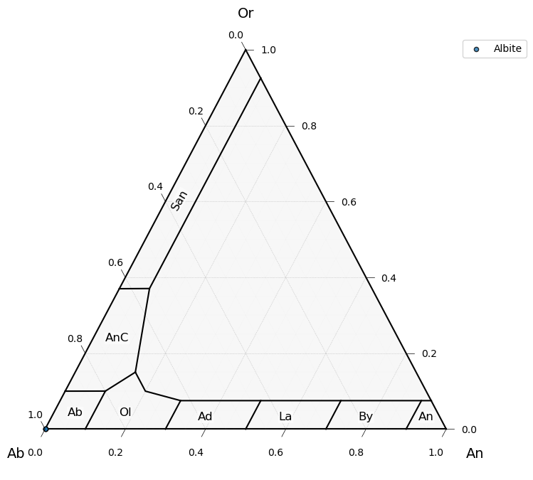
These are albites, and they do indeed plot up in albite space!
Let’s look at the olivines, and calculate up some stoichiometric site occupancies and XFo values!
[10]:
# Use OlivineCalculator to examine stoichiometric/component space (XFo)
ols_comp = mm.OlivineCalculator(ols).calculate_components()
display(ols_comp.head())
| Sample | SiO2 | TiO2 | Al2O3 | FeOt | MnO | MgO | CaO | Na2O | K2O | ... | Predict_Mineral | Prediction_Score | Prediction_Score_Sigma | Second_Predict_Mineral | Second_Prediction_Score | Cation_Sum | M_site | T_site | M_site_expanded | Fo | |
|---|---|---|---|---|---|---|---|---|---|---|---|---|---|---|---|---|---|---|---|---|---|
| 0 | Museum_Ol174.1_highcount_2 | 41.77717 | 0.000017 | 0.005657 | 9.425813 | 0.161341 | 49.51706 | 0.017556 | 0.000013 | 0.005696 | ... | Olivine | 0.996502 | 0.052845 | Nepheline | 0.003324 | 2.989695 | 1.975342 | 1.010146 | 1.979101 | 0.903515 |
| 1 | Museum_Ol174.1_highcount_2 | 41.71127 | 0.000017 | 0.000019 | 9.353550 | 0.121697 | 49.56913 | 0.034175 | 0.003019 | 0.008749 | ... | Olivine | 0.999182 | 0.007934 | Serpentine | 0.000765 | 2.990704 | 1.977335 | 1.009358 | 1.980715 | 0.904275 |
| 2 | Museum_Ol174.1_highcount_2 | 41.74872 | 0.000017 | 0.000019 | 9.297508 | 0.144290 | 49.75990 | 0.011651 | 0.000013 | 0.005699 | ... | Olivine | 0.999268 | 0.007990 | Serpentine | 0.000495 | 2.991556 | 1.979606 | 1.008493 | 1.982860 | 0.905124 |
| 3 | Museum_Ol174.1_highcount_2 | 41.87691 | 0.000017 | 0.000019 | 9.372102 | 0.116922 | 49.71903 | 0.023644 | 0.000013 | 0.000012 | ... | Olivine | 0.992237 | 0.072574 | Apatite | 0.004258 | 2.989806 | 1.976470 | 1.009969 | 1.979469 | 0.904364 |
| 4 | Museum_Ol174.1_highcount_2 | 41.78258 | 0.000017 | 0.003852 | 9.354717 | 0.141731 | 49.81131 | 0.021923 | 0.001326 | 0.003255 | ... | Olivine | 0.999661 | 0.003711 | Serpentine | 0.000211 | 2.991909 | 1.979839 | 1.007899 | 1.983302 | 0.904685 |
5 rows × 57 columns
All the relevant site information (M, T sites) and forsterite content are calculated and returned!
Let’s look at the pyroxenes, and calculate up stoichiometric site occupancies and examine at the component space (En, Wo, Fs).
[11]:
# Use PyroxeneClassifier to examine stoichiometric/component space (En, Wo, Fs).
pxs_comp = mm.PyroxeneClassifier(pxs).calculate_components()
display(pxs_comp.head())

# Use PyroxeneClassifier to plot up these data.
fig = mm.PyroxeneClassifier(pxs).plot()
| Sample | SiO2 | TiO2 | Al2O3 | FeOt | MnO | MgO | CaO | Na2O | K2O | ... | EnFs | DiHd_2003 | Di | Fe3_Wang21 | Fe2_Wang21 | Di_h | Hd_h | Aeg_h | Jd_h | En_h | |
|---|---|---|---|---|---|---|---|---|---|---|---|---|---|---|---|---|---|---|---|---|---|
| 15 | TwinLakesDiopside | 56.7804 | 0.0 | 0.0 | 0.060834 | 0.000698 | 18.4330 | 25.7335 | 0.0 | 0.0 | ... | 0.009220 | 0.960862 | 0.959066 | -0.039877 | 0.041687 | 0.940923 | 0.0 | 0.0 | 0.0 | 0.019200 |
| 16 | TwinLakesDiopside | 56.7965 | 0.0 | 0.0 | 0.062401 | 0.007511 | 18.4492 | 25.7467 | 0.0 | 0.0 | ... | 0.009243 | 0.961270 | 0.959228 | -0.039165 | 0.041020 | 0.941688 | 0.0 | 0.0 | 0.0 | 0.019148 |
| 17 | TwinLakesDiopside | 56.6400 | 0.0 | 0.0 | 0.069621 | 0.004826 | 18.4928 | 25.7743 | 0.0 | 0.0 | ... | 0.008481 | 0.966572 | 0.964392 | -0.033166 | 0.035239 | 0.949988 | 0.0 | 0.0 | 0.0 | 0.016845 |
| 18 | TwinLakesDiopside | 56.7002 | 0.0 | 0.0 | 0.055659 | 0.008368 | 18.4510 | 25.7420 | 0.0 | 0.0 | ... | 0.008763 | 0.963272 | 0.961397 | -0.037097 | 0.038754 | 0.944755 | 0.0 | 0.0 | 0.0 | 0.018148 |
| 19 | TwinLakesDiopside | 56.7272 | 0.0 | 0.0 | 0.059733 | 0.001823 | 18.4430 | 25.7682 | 0.0 | 0.0 | ... | 0.008185 | 0.963722 | 0.961920 | -0.037390 | 0.039168 | 0.945071 | 0.0 | 0.0 | 0.0 | 0.017538 |
5 rows × 86 columns
/home/docs/checkouts/readthedocs.org/user_builds/mineralml/conda/stable/lib/python3.9/site-packages/ternary/plotting.py:148: UserWarning: No data for colormapping provided via 'c'. Parameters 'vmin', 'vmax' will be ignored
  ax.scatter(xs, ys, vmin=vmin, vmax=vmax, **kwargs)
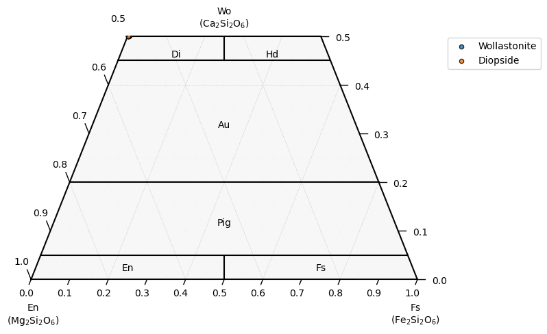
These are diopsides, and they do indeed plot up in diopside space!
Let’s look at the glasses, and calculate up stoichiometric site occupancies and examine them in TAS space.
[12]:
# Use GlassClassifier to return Mg#s and determine the TAS classification.
gls_comp = mm.GlassClassifier(gls).calculate_components()
display(gls_comp)

# Use GlassClassifier to plot up these data.
fig = mm.GlassClassifier(gls).plot()
| SiO2 | TiO2 | Al2O3 | FeOt | MnO | MgO | CaO | Na2O | K2O | P2O5 | ... | K2O_mols | MgO_mols | MnO_mols | Na2O_mols | P2O5_mols | SiO2_mols | TiO2_mols | MgNo | Mineral | TAS | |
|---|---|---|---|---|---|---|---|---|---|---|---|---|---|---|---|---|---|---|---|---|---|
| 30 | 51.5531 | 1.3431 | 15.0794 | 9.2081 | 0.1651 | 8.0553 | 11.0920 | 2.7395 | 0.0719 | 0.0 | ... | 0.000763 | 0.199862 | 0.002327 | 0.044201 | 0.0 | 0.858074 | 0.016817 | 0.609279 | Glass | Basalt |
| 31 | 51.5500 | 1.3190 | 15.0192 | 9.1835 | 0.1710 | 8.0690 | 11.0471 | 2.7411 | 0.0699 | 0.0 | ... | 0.000742 | 0.200201 | 0.002411 | 0.044226 | 0.0 | 0.858023 | 0.016515 | 0.610320 | Glass | Basalt |
| 32 | 51.6652 | 1.3438 | 15.0686 | 9.2527 | 0.1555 | 8.0666 | 11.0889 | 2.7479 | 0.0775 | 0.0 | ... | 0.000823 | 0.200142 | 0.002192 | 0.044336 | 0.0 | 0.859940 | 0.016826 | 0.608462 | Glass | Basalt |
| 33 | 51.6838 | 1.3415 | 15.0678 | 9.2828 | 0.2064 | 8.0310 | 11.0918 | 2.7521 | 0.0809 | 0.0 | ... | 0.000859 | 0.199259 | 0.002910 | 0.044404 | 0.0 | 0.860250 | 0.016797 | 0.606633 | Glass | Basalt |
| 34 | 51.6122 | 1.3448 | 15.0311 | 9.1791 | 0.1597 | 8.0274 | 11.0576 | 2.7345 | 0.0740 | 0.0 | ... | 0.000786 | 0.199169 | 0.002251 | 0.044120 | 0.0 | 0.859058 | 0.016838 | 0.609204 | Glass | Basalt |
5 rows × 28 columns
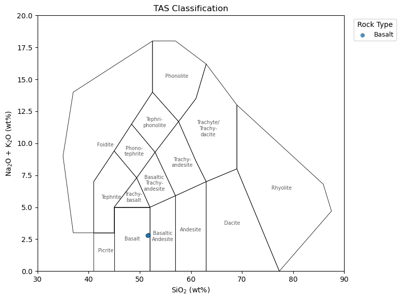
Neat. These are indeed basalts!
5. Perform Thermobarometry
Let’s say that you analyzed these points for thermobarometry, and want to run things through the Thermobar package (Wieser et al., 2022) now. How might you do so? I have written some functions to allow for compatibility with Thermobar, so let’s test things out with some glass analyses as an example.
[13]:
# Filter out the glass from the mineralML prediction in the column, Predict_Mineral. Can also reuse the gls dataframe from above, but remade here for additional reference.
glass = df_pred_nn[df_pred_nn.Predict_Mineral=='Glass']

# Prepare dataframe for thermobarometry by appending the suffix of _Liq to the oxide columns
glass_pt = mm.format_for_thermobar(glass, suffix='_Liq')
display(glass_pt)

# Calculate temperatures with Thermobar, with the Shea et al., 2022 liquid thermometer.
liq_ts = pt.calculate_liq_only_temp(liq_comps=glass_pt,
                                    equationT='T_Shea2022_MgO')
display(liq_ts)
| Sample | SiO2_Liq | TiO2_Liq | Al2O3_Liq | FeOt_Liq | MnO_Liq | MgO_Liq | CaO_Liq | Na2O_Liq | K2O_Liq | Cr2O3_Liq | P2O5_Liq | ZrO2_Liq | Mineral | Predict_Mineral | Prediction_Score | Prediction_Score_Sigma | Second_Predict_Mineral | Second_Prediction_Score | Submineral | |
|---|---|---|---|---|---|---|---|---|---|---|---|---|---|---|---|---|---|---|---|---|
| 30 | Basalt_113716-1_1_WDS | 51.5531 | 1.3431 | 15.0794 | 9.2081 | 0.1651 | 8.0553 | 11.0920 | 2.7395 | 0.0719 | 0.0 | 0.0 | 0.0 | NaN | Glass | 0.997496 | 0.008401 | Amphibole | 0.001572 | NaN |
| 31 | Basalt_113716-1_2_WDS | 51.5500 | 1.3190 | 15.0192 | 9.1835 | 0.1710 | 8.0690 | 11.0471 | 2.7411 | 0.0699 | 0.0 | 0.0 | 0.0 | NaN | Glass | 0.997809 | 0.006814 | Amphibole | 0.001513 | NaN |
| 32 | Basalt_113716-1_3_WDS | 51.6652 | 1.3438 | 15.0686 | 9.2527 | 0.1555 | 8.0666 | 11.0889 | 2.7479 | 0.0775 | 0.0 | 0.0 | 0.0 | NaN | Glass | 0.996068 | 0.026892 | Amphibole | 0.003199 | NaN |
| 33 | Basalt_113716-1_4_WDS | 51.6838 | 1.3415 | 15.0678 | 9.2828 | 0.2064 | 8.0310 | 11.0918 | 2.7521 | 0.0809 | 0.0 | 0.0 | 0.0 | NaN | Glass | 0.998022 | 0.006875 | Amphibole | 0.001234 | NaN |
| 34 | Basalt_113716-1_5_WDS | 51.6122 | 1.3448 | 15.0311 | 9.1791 | 0.1597 | 8.0274 | 11.0576 | 2.7345 | 0.0740 | 0.0 | 0.0 | 0.0 | NaN | Glass | 0.998189 | 0.005033 | Amphibole | 0.001228 | NaN |
30    1460.92236
31    1461.21280
32    1461.16192
33    1460.40720
34    1460.33088
Name: MgO_Liq, dtype: float64
You can do the same thing for any other mineral or melt thermobarometer/chemometer. Append a different suffix for usage with Thermobar! Find one more example of clinopyroxene barometry below.
[14]:
# Filter out the clinopyroxenes from the mineralML prediction in the column, Predict_Mineral. Can also reuse the pxs dataframe from above, but remade here for additional reference.
clinopyroxene = df_pred_nn[df_pred_nn.Predict_Mineral=='Clinopyroxene']

# Prepare dataframe for thermobarometry by appending the suffix of _Cpx to the oxide columns
clinopyroxene_pt = mm.format_for_thermobar(clinopyroxene, suffix='_Cpx')
display(clinopyroxene_pt)

# Calculate temperatures and pressures with Thermobar, with the Putirka, 2008 clinopyroxene thermobarometer.
cpx_ps = pt.calculate_cpx_only_press_temp(cpx_comps=clinopyroxene_pt,
                                          equationT="T_Put2008_eq32d",
                                          equationP="P_Put2008_eq32b",
                                          H2O_Liq=3)
display(cpx_ps)
| Sample | SiO2_Cpx | TiO2_Cpx | Al2O3_Cpx | FeOt_Cpx | MnO_Cpx | MgO_Cpx | CaO_Cpx | Na2O_Cpx | K2O_Cpx | Cr2O3_Cpx | P2O5_Cpx | ZrO2_Cpx | Mineral | Predict_Mineral | Prediction_Score | Prediction_Score_Sigma | Second_Predict_Mineral | Second_Prediction_Score | Submineral | |
|---|---|---|---|---|---|---|---|---|---|---|---|---|---|---|---|---|---|---|---|---|
| 15 | TwinLakesDiopside | 56.7804 | 0.000000 | 0.000000 | 0.060834 | 0.000698 | 18.4330 | 25.7335 | 0.000000 | 0.0 | 0.000000 | 0.0 | 0.0 | NaN | Clinopyroxene | 0.990018 | 0.087620 | Melilite | 0.009753 | Wollastonite |
| 16 | TwinLakesDiopside | 56.7965 | 0.000000 | 0.000000 | 0.062401 | 0.007511 | 18.4492 | 25.7467 | 0.000000 | 0.0 | 0.000000 | 0.0 | 0.0 | NaN | Clinopyroxene | 0.995524 | 0.030773 | Melilite | 0.004396 | Wollastonite |
| 17 | TwinLakesDiopside | 56.6400 | 0.000000 | 0.000000 | 0.069621 | 0.004826 | 18.4928 | 25.7743 | 0.000000 | 0.0 | 0.000000 | 0.0 | 0.0 | NaN | Clinopyroxene | 0.983612 | 0.109517 | Melilite | 0.015668 | Diopside |
| 18 | TwinLakesDiopside | 56.7002 | 0.000000 | 0.000000 | 0.055659 | 0.008368 | 18.4510 | 25.7420 | 0.000000 | 0.0 | 0.002227 | 0.0 | 0.0 | NaN | Clinopyroxene | 0.997114 | 0.021070 | Melilite | 0.002826 | Wollastonite |
| 19 | TwinLakesDiopside | 56.7272 | 0.000000 | 0.000000 | 0.059733 | 0.001823 | 18.4430 | 25.7682 | 0.000000 | 0.0 | 0.003180 | 0.0 | 0.0 | NaN | Clinopyroxene | 0.995375 | 0.025479 | Melilite | 0.003835 | Wollastonite |
| 20 | Diopside_117733_1 | 56.6971 | 0.014333 | 0.230047 | 0.196070 | 0.033566 | 18.1725 | 25.4832 | 0.190501 | 0.0 | 0.003198 | 0.0 | 0.0 | NaN | Clinopyroxene | 0.997084 | 0.016959 | Melilite | 0.002823 | Wollastonite |
| 21 | Diopside_117733_1 | 56.4262 | 0.013831 | 0.228832 | 0.240967 | 0.033234 | 18.0318 | 25.3790 | 0.203233 | 0.0 | 0.000000 | 0.0 | 0.0 | NaN | Clinopyroxene | 0.996425 | 0.029234 | Melilite | 0.003442 | Wollastonite |
| 22 | Diopside_117733_1 | 56.4609 | 0.013084 | 0.203597 | 0.261528 | 0.030660 | 18.0912 | 25.4615 | 0.173151 | 0.0 | 0.000000 | 0.0 | 0.0 | NaN | Clinopyroxene | 0.997756 | 0.010260 | Melilite | 0.002175 | Wollastonite |
| 23 | Diopside_117733_1 | 56.7182 | 0.009387 | 0.204781 | 0.249543 | 0.029107 | 18.1683 | 25.5439 | 0.164830 | 0.0 | 0.003649 | 0.0 | 0.0 | NaN | Clinopyroxene | 0.994745 | 0.034862 | Melilite | 0.003266 | Wollastonite |
| 24 | Diopside_117733_1 | 56.6649 | 0.009884 | 0.205739 | 0.260411 | 0.029596 | 18.1841 | 25.5244 | 0.170126 | 0.0 | 0.000000 | 0.0 | 0.0 | NaN | Clinopyroxene | 0.991305 | 0.064455 | Melilite | 0.008551 | Wollastonite |
| P_kbar_calc | T_K_calc | Delta_P_kbar_Iter | Delta_T_K_Iter | Sample | SiO2_Cpx | TiO2_Cpx | Al2O3_Cpx | FeOt_Cpx | MnO_Cpx | ... | Jd_from 0=Na, 1=Al | Jd | CaTs | CaTi | DiHd_1996 | EnFs | DiHd_2003 | Di_Cpx | FeIII_Wang21 | FeII_Wang21 | |
|---|---|---|---|---|---|---|---|---|---|---|---|---|---|---|---|---|---|---|---|---|---|
| 15 | NaN | NaN | NaN | NaN | NaN | 56.7804 | 0.000000 | 0.000000 | 0.060834 | 0.000698 | ... | 0 | 0.000000 | 0.019891 | 0.0 | 0.960956 | 0.009196 | 0.960956 | 0.959160 | -0.039783 | 0.041592 |
| 16 | NaN | NaN | NaN | NaN | NaN | 56.7965 | 0.000000 | 0.000000 | 0.062401 | 0.007511 | ... | 0 | 0.000000 | 0.019535 | 0.0 | 0.961364 | 0.009220 | 0.961364 | 0.959322 | -0.039070 | 0.040926 |
| 17 | NaN | NaN | NaN | NaN | NaN | 56.6400 | 0.000000 | 0.000000 | 0.069621 | 0.004826 | ... | 0 | 0.000000 | 0.016536 | 0.0 | 0.966666 | 0.008457 | 0.966666 | 0.964486 | -0.033072 | 0.035144 |
| 18 | NaN | NaN | NaN | NaN | NaN | 56.7002 | 0.000000 | 0.000000 | 0.055659 | 0.008368 | ... | 0 | 0.000000 | 0.018470 | 0.0 | 0.963367 | 0.008739 | 0.963367 | 0.961492 | -0.037003 | 0.038660 |
| 19 | NaN | NaN | NaN | NaN | NaN | 56.7272 | 0.000000 | 0.000000 | 0.059733 | 0.001823 | ... | 0 | 0.000000 | 0.018603 | 0.0 | 0.963816 | 0.008162 | 0.963816 | 0.962015 | -0.037296 | 0.039074 |
| 20 | -2.682948 | 1344.722303 | 0.0 | 0.0 | NaN | 56.6971 | 0.014333 | 0.230047 | 0.196070 | 0.033566 | ... | 0 | 0.013144 | 0.014215 | 0.0 | 0.957424 | 0.006255 | 0.957424 | 0.950672 | -0.032784 | 0.038619 |
| 21 | -2.643540 | 1336.833754 | 0.0 | 0.0 | NaN | 56.4262 | 0.013831 | 0.228832 | 0.240967 | 0.033234 | ... | 0 | 0.014092 | 0.013441 | 0.0 | 0.959001 | 0.004758 | 0.959001 | 0.950877 | -0.032074 | 0.039280 |
| 22 | -3.239814 | 1332.217801 | 0.0 | 0.0 | NaN | 56.4609 | 0.013084 | 0.203597 | 0.261528 | 0.030660 | ... | 0 | 0.011992 | 0.013467 | 0.0 | 0.961054 | 0.005083 | 0.961054 | 0.952413 | -0.031057 | 0.038870 |
| 23 | -3.176065 | 1339.951742 | 0.0 | 0.0 | NaN | 56.7182 | 0.009387 | 0.204781 | 0.249543 | 0.029107 | ... | 0 | 0.011369 | 0.014896 | 0.0 | 0.958674 | 0.006126 | 0.958674 | 0.950485 | -0.033179 | 0.040603 |
| 24 | -3.157676 | 1339.323094 | 0.0 | 0.0 | NaN | 56.6649 | 0.009884 | 0.205739 | 0.260411 | 0.029596 | ... | 0 | 0.011740 | 0.013763 | 0.0 | 0.959641 | 0.006486 | 0.959641 | 0.951120 | -0.031165 | 0.038917 |
10 rows × 58 columns
Note that the first 5 analyses do not have any Na2O and thus no jadeite component, so they return pressures of NaNs (cannot get a pressure from this clinopyroxene).
Hopefully, this sort of workflow can facilitate certainty in mineralogy prior to performing thermobarometry!