This page was generated from
docs/examples/mineralML_neuralnetwork.ipynb.
Interactive online version:
![]() .
.
[1]:
""" Created on November 13, 2023 // Updated on March 20, 2026 // @author: Sarah Shi """

import os
import numpy as np
import pandas as pd

import mineralML as mm
from sklearn.metrics import classification_report

import matplotlib.pyplot as plt
%matplotlib inline
%config InlineBackend.figure_format = 'png'
mineralML Quickstart for Tabular Data
This notebook shows how to load and run your data through mineralML with an example CSV: training_hundred.csv. This is a five step process:
Load a CSV with
mm.load_df(orpd.read_csvdirectly). Clean and align columns withmm.prep_df.Run data through the neural network with
mm.predict_class_probto derive classifications and prediction scores.Export prediction scores with
mm.export_predictions_to_excel.Examine predictions with
classification_report,mm.confusion_matrix_df, andmm.pp_matrix.Project data into latent space with
mm.plot_latent_space, for visualization.
We loaded in the mineralML Python package as mm. mineralML has trained machine learning models for classifying minerals. This implementation aims to get your electron microprobe or quantitative EDS compositions classified and processed. We remove some degrees of freedom to simplify the process as much as possible. The minerals considered for this study include: Amphibole, Apatite, Biotite, Calcite, Chlorite, Epidote, Feldspar (Alkali Feldspar and Plagioclase), Garnet, Glass,
Kalsilite, Leucite, Melilite, Muscovite, Nepheline, Olivine, Oxide (Rhombohedral_Oxides including Hematite-Ilmenite, Spinel_Group including Magnetite-Spinel), Pyroxene (Clinopyroxene, Orthopyroxene, Na-Pyroxene), Quartz, Rutile, Serpentine, Titanite, Tourmaline, and Zircon.
One CSV file containing your electron microprobe analyses in oxide weight percentages is necessary. Find an example here. The necessary oxides are SiO\(_2\), TiO\(_2\), Al\(_2\)O\(_3\), FeO\(_t\), MnO, MgO, CaO, Na\(_2\)O, K\(_2\)O, Cr\(_2\)O\(_3\), P\(_2\)O\(_5\), and ZrO\(_2\) (if you are aiming to classify zircon). For the oxides not analyzed for specific minerals, the preprocessing will fill in the nan values as 0.
We will apply the neural network method to the dataset.
1. Load and prepare data for analysis
We will use mm.load_df and mm.prep_df to do so.
[2]:
# Read in your dataframe of mineral data, called training_hundred.csv.
df_load = mm.load_df('TabularData/training_hundred.csv')

# Prepare the dataframe by removing rows with too many NaNs, and filling in zeros.
df_nn = mm.prep_df(df_load, # dataframe to prepare
                   renormalize=False, # optionally renormalize rows to sum to 100 wt%
                   convert_fe=False, # optionally convert disparate input formats of Fe all to FeOt
                   drop_empty_rows=False, # optionally drop rows with more nan values than the min_oxide_count
                   min_oxide_count=2, # minimum number of oxides in a row to keep that analysis
                   verbose=True
                   )
prep_df: 2800 row(s) processed (of 2800 input, 0 dropped).
[3]:
# Examine the prepared dataframe

display(df_nn.head())
| Sample Name | SiO2 | TiO2 | Al2O3 | FeOt | MnO | MgO | CaO | Na2O | K2O | Cr2O3 | P2O5 | ZrO2 | Mineral | Source | |
|---|---|---|---|---|---|---|---|---|---|---|---|---|---|---|---|
| 0 | Z2099 | 42.96 | 1.80 | 14.33 | 4.07 | 0.07 | 17.39 | 12.03 | 3.10 | 0.03 | 0.65 | 0.0 | 0.0 | Amphibole | Vannuccietal1995 |
| 1 | Z2070 | 43.03 | 2.39 | 13.35 | 4.09 | 0.06 | 17.01 | 11.71 | 2.97 | 0.05 | 0.74 | 0.0 | 0.0 | Amphibole | Vannuccietal1995 |
| 2 | Z2073 | 42.95 | 3.02 | 14.12 | 4.35 | 0.06 | 17.53 | 12.02 | 3.04 | 0.07 | 0.76 | 0.0 | 0.0 | Amphibole | Vannuccietal1995 |
| 3 | Z2067 | 43.01 | 4.65 | 12.83 | 4.39 | 0.07 | 17.14 | 12.14 | 2.88 | 0.03 | 0.84 | 0.0 | 0.0 | Amphibole | Vannuccietal1995 |
| 4 | Z2068 | 42.13 | 4.87 | 12.15 | 4.08 | 0.05 | 16.42 | 11.89 | 2.75 | 0.02 | 1.26 | 0.0 | 0.0 | Amphibole | Vannuccietal1995 |
2. Apply the trained neural network (mm.predict_class_prob)
We will use mm.predict_class_prob to do so.
[4]:
# The trained neural network can be applied in just one line. It returns predictions in columns called "Predict_Mineral", "Submineral" (if applicable, for pyroxenes, feldspars, and oxides), "Predict_Probability", "Second_Predict_Mineral", "Second_Predict_Probability".

df_pred_nn = mm.predict_class_prob(df_nn)
mineralML: 2800 rows — 2500 classified by neural network, 300 by empirical rules (Zircon: 100, SiO2 polymorph: 100, Carbonate: 100), 0 skipped (invalid/empty)
[5]:
# Examine the predicted mineral classifications

display(df_pred_nn)
| Sample Name | SiO2 | TiO2 | Al2O3 | FeOt | MnO | MgO | CaO | Na2O | K2O | ... | P2O5 | ZrO2 | Mineral | Source | Predict_Mineral | Prediction_Score | Prediction_Score_Sigma | Second_Predict_Mineral | Second_Prediction_Score | Submineral | |
|---|---|---|---|---|---|---|---|---|---|---|---|---|---|---|---|---|---|---|---|---|---|
| 0 | Z2099 | 42.96 | 1.80 | 14.33 | 4.07 | 0.07 | 17.39 | 12.03 | 3.10 | 0.03 | ... | 0.00 | 0.0 | Amphibole | Vannuccietal1995 | Amphibole | 0.987575 | 0.036975 | Pyroxene | 0.004594 | NaN |
| 1 | Z2070 | 43.03 | 2.39 | 13.35 | 4.09 | 0.06 | 17.01 | 11.71 | 2.97 | 0.05 | ... | 0.00 | 0.0 | Amphibole | Vannuccietal1995 | Amphibole | 0.992861 | 0.019478 | Pyroxene | 0.002798 | NaN |
| 2 | Z2073 | 42.95 | 3.02 | 14.12 | 4.35 | 0.06 | 17.53 | 12.02 | 3.04 | 0.07 | ... | 0.00 | 0.0 | Amphibole | Vannuccietal1995 | Amphibole | 0.991113 | 0.018898 | Pyroxene | 0.004357 | NaN |
| 3 | Z2067 | 43.01 | 4.65 | 12.83 | 4.39 | 0.07 | 17.14 | 12.14 | 2.88 | 0.03 | ... | 0.00 | 0.0 | Amphibole | Vannuccietal1995 | Amphibole | 0.992671 | 0.015184 | Pyroxene | 0.003859 | NaN |
| 4 | Z2068 | 42.13 | 4.87 | 12.15 | 4.08 | 0.05 | 16.42 | 11.89 | 2.75 | 0.02 | ... | 0.00 | 0.0 | Amphibole | Vannuccietal1995 | Amphibole | 0.993189 | 0.017474 | Pyroxene | 0.003345 | NaN |
| ... | ... | ... | ... | ... | ... | ... | ... | ... | ... | ... | ... | ... | ... | ... | ... | ... | ... | ... | ... | ... | ... |
| 2795 | 23B-03 | 50.39 | 1.71 | 13.95 | 12.55 | 0.22 | 6.90 | 11.78 | 2.41 | 0.33 | ... | 0.15 | 0.0 | Glass | Hartleyetal2013 | Glass | 0.997337 | 0.009643 | Amphibole | 0.001483 | NaN |
| 2796 | 23B-04 | 49.30 | 1.66 | 13.99 | 11.94 | 0.21 | 7.16 | 12.04 | 2.16 | 0.32 | ... | 0.15 | 0.0 | Glass | Hartleyetal2013 | Glass | 0.996660 | 0.015642 | Amphibole | 0.002413 | NaN |
| 2797 | 23B-04 | 49.73 | 1.61 | 13.63 | 12.15 | 0.21 | 7.13 | 11.90 | 2.30 | 0.33 | ... | 0.16 | 0.0 | Glass | Hartleyetal2013 | Glass | 0.995411 | 0.017832 | Amphibole | 0.003209 | NaN |
| 2798 | 23B-04 | 49.55 | 1.55 | 14.07 | 11.90 | 0.21 | 7.12 | 11.95 | 2.31 | 0.31 | ... | 0.17 | 0.0 | Glass | Hartleyetal2013 | Glass | 0.996472 | 0.011110 | Amphibole | 0.002610 | NaN |
| 2799 | 23B-04 | 49.67 | 1.67 | 13.46 | 11.90 | 0.21 | 7.15 | 11.87 | 2.34 | 0.29 | ... | 0.16 | 0.0 | Glass | Hartleyetal2013 | Glass | 0.995961 | 0.011270 | Amphibole | 0.003020 | NaN |
2800 rows × 21 columns
There is a good amount of information in this dataframe. The predicted mineral is provided in the Predict_Mineral column, along with the prediction score expressed in the Prediction_Score column (representing likelihood of prediction) and standard deviation on this prediction in the Prediction_Score_Sigma column.
3. Export prediction results
Say you would like to go back to working with Excel now. Use mm.export_predictions_to_excel to export the predictions and these values. All the original input data are returned in the first sheet, and data are split into individual mineral phases in all other sheets.
[6]:
# Export prediction results to an Excel workbook with one sheet called "All" containing all rows, and additional sheets for each predicted mineral.

mm.export_predictions_to_excel(df_pred_nn, filename='TabularData/prediction_results.xlsx')
[6]:
'TabularData/prediction_results.xlsx'
4. Examine prediction results
[7]:
# Create a classification report to determine the accuracy, precision, f1, etc. This is possible in this case because these are our training data, where we know the classes.

bayes_valid_report = classification_report(
    df_pred_nn['Mineral'], df_pred_nn['Predict_Mineral'], zero_division=0
)
print("Validation Report:\n", bayes_valid_report)
Validation Report:
                  precision    recall  f1-score   support

Alkali_Feldspar       1.00      1.00      1.00       100
      Amphibole       1.00      0.98      0.99       100
        Apatite       1.00      1.00      1.00       100
        Biotite       1.00      1.00      1.00       100
      Carbonate       1.00      1.00      1.00       100
       Chlorite       1.00      1.00      1.00       100
  Clinopyroxene       0.94      1.00      0.97       100
        Epidote       1.00      1.00      1.00       100
         Garnet       1.00      1.00      1.00       100
          Glass       1.00      1.00      1.00       100
       Hematite       0.00      0.00      0.00       100
       Ilmenite       0.00      0.00      0.00       100
      Kalsilite       1.00      1.00      1.00       100
        Leucite       1.00      1.00      1.00       100
      Magnetite       0.00      0.00      0.00       100
       Melilite       1.00      1.00      1.00       100
      Muscovite       1.00      1.00      1.00       100
      Nepheline       1.00      1.00      1.00       100
        Olivine       1.00      1.00      1.00       100
  Orthopyroxene       1.00      0.96      0.98       100
          Oxide       0.00      0.00      0.00         0
    Plagioclase       1.00      1.00      1.00       100
         Rutile       1.00      1.00      1.00       100
     Serpentine       1.00      1.00      1.00       100
 SiO2_Polymorph       1.00      1.00      1.00       100
         Spinel       0.00      0.00      0.00       100
       Titanite       1.00      1.00      1.00       100
     Tourmaline       1.00      1.00      1.00       100
         Zircon       1.00      1.00      1.00       100

       accuracy                           0.85      2800
      macro avg       0.83      0.83      0.83      2800
   weighted avg       0.86      0.85      0.86      2800
[8]:
# Create and plot a confusion matrix

# This compares your stated mineral and mineralML's predicted mineral
cm = mm.confusion_matrix_df(df_pred_nn['Mineral'], df_pred_nn['Predict_Mineral'])
# This plots the results in a confusion matrix
mm.pp_matrix(cm, figsize=[8, 8], savefig=None)
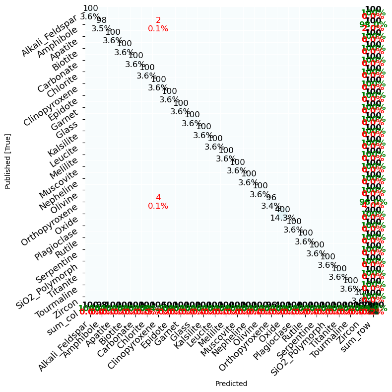
5. Plot in latent space
Excellent, these classifications are quite promising. The most likely predicted minerals, along with their associated prediction scores with uncertainties are returned. We can further visualize these classifications in latent space with mm.plot_latent_space.
[9]:
mm.plot_latent_space(df_pred_nn)
/tmp/ipykernel_3522/3724615771.py:1: UserWarning: Skipping 300 point(s) with labels that do not map to training classes.
  Empirical labels not in neural network classes (expected): {'SiO2_Polymorph', 'Carbonate', 'Zircon'}
  mm.plot_latent_space(df_pred_nn)
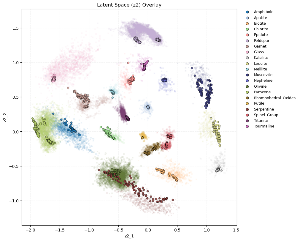
Neat! We can see where these compositions lie in latent space, and whether the predictions line up with our expected mineral phase. The points in the background are from the training and validation dataset.