This page was generated from
docs/examples/mineralML_stoichiometry.ipynb.
Interactive online version:
![]() .
.
[1]:
""" Created on August 22, 2025 // Updated on March 20, 2026 // @author: Sarah Shi """

import os
import numpy as np
import pandas as pd
import matplotlib.pyplot as plt

import mineralML as mm

%matplotlib inline
%config InlineBackend.figure_format = 'png'
mineralML Stoichiometry Calculations
This notebook demonstrates how to use the stoichiometry calculators and classifiers defined in mineralML:
Load and prepare data for analysis
Calculate stoichiometry with
BaseMineralCalculator, for moles, oxygens, cations on a fixed oxygen basisApply specialized calculators for different mineral groups
Perform empirical classifications consistent with petrologist-defined schemes
We loaded in the mineralML Python package as mm. mineralML has trained machine learning models for classifying minerals. This implementation aims to get your electron microprobe or quantitative EDS compositions classified and processed. We remove some degrees of freedom to simplify the process as much as possible. The minerals considered for this study include: Amphibole, Apatite, Biotite, Calcite, Chlorite, Epidote, Feldspar (Alkali Feldspar and Plagioclase), Garnet, Glass,
Kalsilite, Leucite, Melilite, Muscovite, Nepheline, Olivine, Oxide (Rhombohedral_Oxides including Hematite-Ilmenite, Spinel_Group including Magnetite-Spinel), Pyroxene (Clinopyroxene, Orthopyroxene, Na-Pyroxene), Quartz, Rutile, Serpentine, Titanite, Tourmaline, and Zircon.
One CSV file containing your electron microprobe analyses in oxide weight percentages is necessary. Find an example here. The necessary oxides are SiO\(_2\), TiO\(_2\), Al\(_2\)O\(_3\), FeO\(_t\), MnO, MgO, CaO, Na\(_2\)O, K\(_2\)O, Cr\(_2\)O\(_3\), P\(_2\)O\(_5\), and ZrO\(_2\) (if you are aiming to classify zircon). For the oxides not analyzed for specific minerals, the preprocessing will fill in the nan values as 0.
BaseMineralCalculator
``mm.BaseMineralCalculator`` forms the foundation for all stoichiometry workflows in mineralML. It provides the core methods to:
Normalize oxide compositions to a fixed oxygen basis
Convert weight% oxides to moles, oxygens, and cations
Enforce Fe input consistency (FeOt, Fe₂O₃t, or paired FeO/Fe₂O₃)
It returns results in a consistent format:
_mols_ox_cat_{oxbasis}ox— cations per n oxygens
All mineral-specific calculators (e.g., AmphiboleCalculator, FeldsparCalculator, OlivineCalculator, PyroxeneCalculator) inherit from this base. They extend it with additional logic for site allocation, normalization rules, or classification schemes. For most users, no direct interaction is needed with BaseMineralCalculator, but it is useful to know that every group-specific tool builds on this common calculator.
1. Load and prepare data for analysis
[2]:
# Read in your dataframe of mineral data, called training_hundred.csv.
df_load = mm.load_df('TabularData/training_hundred.csv')
display(df_load.head())
| Sample Name | SiO2 | TiO2 | Al2O3 | FeOt | MnO | MgO | CaO | Na2O | K2O | P2O5 | Cr2O3 | ZrO2 | Mineral | Source | |
|---|---|---|---|---|---|---|---|---|---|---|---|---|---|---|---|
| 0 | Z2099 | 42.96 | 1.80 | 14.33 | 4.07 | 0.07 | 17.39 | 12.03 | 3.10 | 0.03 | NaN | 0.65 | NaN | Amphibole | Vannuccietal1995 |
| 1 | Z2070 | 43.03 | 2.39 | 13.35 | 4.09 | 0.06 | 17.01 | 11.71 | 2.97 | 0.05 | NaN | 0.74 | NaN | Amphibole | Vannuccietal1995 |
| 2 | Z2073 | 42.95 | 3.02 | 14.12 | 4.35 | 0.06 | 17.53 | 12.02 | 3.04 | 0.07 | NaN | 0.76 | NaN | Amphibole | Vannuccietal1995 |
| 3 | Z2067 | 43.01 | 4.65 | 12.83 | 4.39 | 0.07 | 17.14 | 12.14 | 2.88 | 0.03 | NaN | 0.84 | NaN | Amphibole | Vannuccietal1995 |
| 4 | Z2068 | 42.13 | 4.87 | 12.15 | 4.08 | 0.05 | 16.42 | 11.89 | 2.75 | 0.02 | NaN | 1.26 | NaN | Amphibole | Vannuccietal1995 |
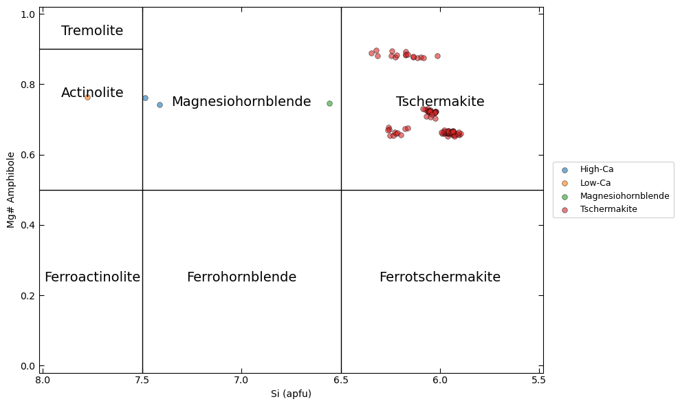
AmphiboleCalculator and AmphiboleClassifier
``mm.AmphiboleCalculator`` and ``mm.AmphiboleClassifier`` perform basic calculations associated with amphibole-group minerals along with site allocations (:cite:t:Leakeetal1997 and :cite:t:Ridolfi2021 from Thermobar :cite:p:Wieseretal2022), and additionally plots these data in a classification diagram. mineralML adds on to the Thermobar classification by also classifying amphiboles on the :cite:t:Leakeetal1997 calcic amphibole classification diagram and
explicitly returning the corresponding Submineral, or the specific type of calcic amphibole.
[3]:
# Let's select just the amphiboles from the training dataset
amp = df_load[df_load.Mineral=='Amphibole']
amp_calc = mm.AmphiboleCalculator(amp)
amp_comp = amp_calc.calculate_components()
[4]:
# Let's print all the columns in this dataframe, along with the compositions returned.
print(list(amp_comp.columns))
display(amp_comp.head())
['Sample', 'SiO2', 'TiO2', 'Al2O3', 'FeOt', 'MnO', 'MgO', 'CaO', 'Na2O', 'K2O', 'P2O5', 'Cr2O3', 'SiO2_mols', 'TiO2_mols', 'Al2O3_mols', 'FeOt_mols', 'MnO_mols', 'MgO_mols', 'CaO_mols', 'Na2O_mols', 'K2O_mols', 'P2O5_mols', 'Cr2O3_mols', 'SiO2_ox', 'TiO2_ox', 'Al2O3_ox', 'FeOt_ox', 'MnO_ox', 'MgO_ox', 'CaO_ox', 'Na2O_ox', 'K2O_ox', 'P2O5_ox', 'Cr2O3_ox', 'Si_cat_23ox', 'Ti_cat_23ox', 'Al_cat_23ox', 'Fe2t_cat_23ox', 'Mn_cat_23ox', 'Mg_cat_23ox', 'Ca_cat_23ox', 'Na_cat_23ox', 'K_cat_23ox', 'P_cat_23ox', 'Cr_cat_23ox', 'Mineral', 'Source', 'Predict_Mineral', 'Prediction_Score', 'Prediction_Score_Sigma', 'Second_Predict_Mineral', 'Second_Prediction_Score', 'Cation_Sum', 'Cation_Sum_Si_Mg', 'Cation_Sum_Si_Ca', 'Cation_Sum_Amp', 'Mgno', 'H2O_calc', 'O=F,Cl', 'Charge', 'Fe3_calc', 'Fe2_calc', 'Fe2O3_calc', 'FeO_calc', 'Sum_input', 'Total_recalc', 'Fail Msg', 'Input_Check', 'Fe2_C', 'Mgno_Fe2', 'Mgno_FeT', 'Ca_B', 'Na_calc', 'B_Sum', 'Na_A', 'K_A', 'A_Sum', 'Classification', 'Cation_Sum_ridolfi', 'Cation_Sum_Si_Mg_ridolfi', 'Cation_Sum_Si_Ca_ridolfi', 'Cation_Sum_Amp_ridolfi', 'Mgno_ridolfi', 'H2O_calc_ridolfi', 'O=F,Cl_ridolfi', 'Charge_ridolfi', 'Fe3_calc_ridolfi', 'Fe2_calc_ridolfi', 'Fe2O3_calc_ridolfi', 'FeO_calc_ridolfi', 'Sum_input_ridolfi', 'Total_recalc_ridolfi', 'Fail Msg_ridolfi', 'Input_Check_ridolfi', 'Fe2_C_ridolfi', 'Mgno_Fe2_ridolfi', 'Mgno_FeT_ridolfi', 'Ca_B_ridolfi', 'Na_calc_ridolfi', 'B_Sum_ridolfi', 'Na_A_ridolfi', 'K_A_ridolfi', 'A_Sum_ridolfi', 'Classification_ridolfi', 'Si_13cat_ridolfi_norm', 'Ti_13cat_ridolfi_norm', 'Al_13cat_ridolfi_norm', 'Fe2t_13cat_ridolfi_norm', 'Mn_13cat_ridolfi_norm', 'Mg_13cat_ridolfi_norm', 'Ca_13cat_ridolfi_norm', 'Na_13cat_ridolfi_norm', 'K_13cat_ridolfi_norm', 'P_13cat_ridolfi_norm', 'Cr_13cat_ridolfi_norm', 'Si_T_leake', 'Al_T_leake', 'Al_C_leake', 'Ti_C_leake', 'Mg_C_leake', 'Fe2t_C_leake', 'Mn_C_leake', 'Cr_C_leake', 'Mg_B_leake', 'Fe2t_B_leake', 'Mn_B_leake', 'Na_B_leake', 'Ca_B_leake', 'Na_A_leake', 'K_A_leake', 'Ca_A_leake', 'Sum_T_leake', 'Sum_C_leake', 'Sum_B_leake', 'Sum_A_leake', 'Cation_Sum_leake', 'Mgno_leake']
| Sample | SiO2 | TiO2 | Al2O3 | FeOt | MnO | MgO | CaO | Na2O | K2O | ... | Ca_B_leake | Na_A_leake | K_A_leake | Ca_A_leake | Sum_T_leake | Sum_C_leake | Sum_B_leake | Sum_A_leake | Cation_Sum_leake | Mgno_leake | |
|---|---|---|---|---|---|---|---|---|---|---|---|---|---|---|---|---|---|---|---|---|---|
| 0 | Z2099 | 42.96 | 1.80 | 14.33 | 4.07 | 0.07 | 17.39 | 12.03 | 3.10 | 0.03 | ... | 1.852409 | 0.809623 | 0.005500 | 0.0 | 8.0 | 4.805388 | 2.0 | 0.815124 | 15.620512 | 0.883941 |
| 1 | Z2070 | 43.03 | 2.39 | 13.35 | 4.09 | 0.06 | 17.01 | 11.71 | 2.97 | 0.05 | ... | 1.821486 | 0.720368 | 0.009260 | 0.0 | 8.0 | 4.738969 | 2.0 | 0.729629 | 15.468597 | 0.881142 |
| 2 | Z2073 | 42.95 | 3.02 | 14.12 | 4.35 | 0.06 | 17.53 | 12.02 | 3.04 | 0.07 | ... | 1.828409 | 0.767508 | 0.012678 | 0.0 | 8.0 | 4.677446 | 2.0 | 0.780186 | 15.457632 | 0.877802 |
| 3 | Z2067 | 43.01 | 4.65 | 12.83 | 4.39 | 0.07 | 17.14 | 12.14 | 2.88 | 0.03 | ... | 1.848999 | 0.660659 | 0.005440 | 0.0 | 8.0 | 4.502725 | 2.0 | 0.666100 | 15.168824 | 0.874366 |
| 4 | Z2068 | 42.13 | 4.87 | 12.15 | 4.08 | 0.05 | 16.42 | 11.89 | 2.75 | 0.02 | ... | 1.855450 | 0.632008 | 0.003716 | 0.0 | 8.0 | 4.435406 | 2.0 | 0.635724 | 15.071130 | 0.877658 |
5 rows × 137 columns
[5]:
# Now, let's classify and plot up these amphiboles.
amp_class = mm.AmphiboleClassifier(amp)
amp_comp_class = amp_class.classify()

# Note the addition of the Submineral column providing a calcic amphibole classification.
display(amp_comp_class.head())
/tmp/ipykernel_3627/3864048812.py:3: UserWarning: 1 row(s) have Ca_B < 1.5 and are not calcic amphiboles. The Leake classifier only covers calcic amphiboles; these rows will not be sub-classified in the ternary diagram.
  amp_comp_class = amp_class.classify()
/tmp/ipykernel_3627/3864048812.py:3: UserWarning: 2 row(s) have Ca_B > 2.05 and fall outside the calcic amphibole domain. These rows will not be sub-classified in the ternary diagram.
  amp_comp_class = amp_class.classify()
| Sample | SiO2 | TiO2 | Al2O3 | FeOt | MnO | MgO | CaO | Na2O | K2O | ... | Na_A_leake | K_A_leake | Ca_A_leake | Sum_T_leake | Sum_C_leake | Sum_B_leake | Sum_A_leake | Cation_Sum_leake | Mgno_leake | Submineral | |
|---|---|---|---|---|---|---|---|---|---|---|---|---|---|---|---|---|---|---|---|---|---|
| 0 | Z2099 | 42.96 | 1.80 | 14.33 | 4.07 | 0.07 | 17.39 | 12.03 | 3.10 | 0.03 | ... | 0.809623 | 0.005500 | 0.0 | 8.0 | 4.805388 | 2.0 | 0.815124 | 15.620512 | 0.883941 | Tschermakite |
| 1 | Z2070 | 43.03 | 2.39 | 13.35 | 4.09 | 0.06 | 17.01 | 11.71 | 2.97 | 0.05 | ... | 0.720368 | 0.009260 | 0.0 | 8.0 | 4.738969 | 2.0 | 0.729629 | 15.468597 | 0.881142 | Tschermakite |
| 2 | Z2073 | 42.95 | 3.02 | 14.12 | 4.35 | 0.06 | 17.53 | 12.02 | 3.04 | 0.07 | ... | 0.767508 | 0.012678 | 0.0 | 8.0 | 4.677446 | 2.0 | 0.780186 | 15.457632 | 0.877802 | Tschermakite |
| 3 | Z2067 | 43.01 | 4.65 | 12.83 | 4.39 | 0.07 | 17.14 | 12.14 | 2.88 | 0.03 | ... | 0.660659 | 0.005440 | 0.0 | 8.0 | 4.502725 | 2.0 | 0.666100 | 15.168824 | 0.874366 | Tschermakite |
| 4 | Z2068 | 42.13 | 4.87 | 12.15 | 4.08 | 0.05 | 16.42 | 11.89 | 2.75 | 0.02 | ... | 0.632008 | 0.003716 | 0.0 | 8.0 | 4.435406 | 2.0 | 0.635724 | 15.071130 | 0.877658 | Tschermakite |
5 rows × 138 columns
[6]:
# Here, we can plot up these amphiboles.
fig, ax = amp_class.plot()
/home/docs/checkouts/readthedocs.org/user_builds/mineralml/checkouts/stable/src/mineralML/stoichiometry.py:687: UserWarning: 1 row(s) have Ca_B < 1.5 and are not calcic amphiboles. The Leake classifier only covers calcic amphiboles; these rows will not be sub-classified in the ternary diagram.
  df_class = self.classify(subclass=subclass)
/home/docs/checkouts/readthedocs.org/user_builds/mineralml/checkouts/stable/src/mineralML/stoichiometry.py:687: UserWarning: 2 row(s) have Ca_B > 2.05 and fall outside the calcic amphibole domain. These rows will not be sub-classified in the ternary diagram.
  df_class = self.classify(subclass=subclass)
ApatiteCalculator
``mm.ApatiteCalculator`` performs basic calculations and site allocations associated with apatite-group minerals.
[7]:
ap = df_load[df_load.Mineral=='Apatite']
ap_calc = mm.ApatiteCalculator(ap)
ap_comp = ap_calc.calculate_components()
display(ap_comp.head())
| Sample | SiO2 | TiO2 | Al2O3 | FeOt | MnO | MgO | CaO | Na2O | K2O | ... | Source | Predict_Mineral | Prediction_Score | Prediction_Score_Sigma | Second_Predict_Mineral | Second_Prediction_Score | Cation_Sum | M_site | T_site | Ca_P | |
|---|---|---|---|---|---|---|---|---|---|---|---|---|---|---|---|---|---|---|---|---|---|
| 100 | SG-09-32_12 | 0.17 | NaN | NaN | 0.70 | NaN | 0.13 | 54.32 | NaN | NaN | ... | Scottetal2015 | NaN | NaN | NaN | NaN | NaN | 8.353343 | 5.181160 | 3.102816 | 8.268841 |
| 101 | SG-09-32_23 | 0.14 | NaN | NaN | 0.61 | NaN | 0.20 | 53.52 | NaN | NaN | ... | Scottetal2015 | NaN | NaN | NaN | NaN | NaN | 8.321227 | 5.125625 | 3.123353 | 8.236464 |
| 102 | SG-09-32_32 | 0.24 | NaN | NaN | 0.56 | NaN | 0.21 | 53.53 | NaN | NaN | ... | Scottetal2015 | NaN | NaN | NaN | NaN | NaN | 8.341031 | 5.157591 | 3.113174 | 8.249181 |
| 103 | 2006-69_65 | 0.13 | NaN | NaN | 0.45 | NaN | 0.24 | 53.67 | NaN | NaN | ... | Scottetal2015 | NaN | NaN | NaN | NaN | NaN | 8.399179 | 5.260840 | 3.071178 | 8.320124 |
| 104 | 2006-69_70 | 0.20 | NaN | NaN | 0.74 | NaN | 0.23 | 53.86 | NaN | NaN | ... | Scottetal2015 | NaN | NaN | NaN | NaN | NaN | 8.341776 | 5.144612 | 3.111426 | 8.238207 |
5 rows × 56 columns
BiotiteCalculator
``mm.BiotiteCalculator`` performs basic calculations and site allocations associated with biotite-group minerals.
[8]:
bt = df_load[df_load.Mineral=='Biotite']
bt_calc = mm.BiotiteCalculator(bt)
bt_comp = bt_calc.calculate_components()
display(bt_comp.head())
| Sample | SiO2 | TiO2 | Al2O3 | FeOt | MnO | MgO | CaO | Na2O | K2O | ... | Predict_Mineral | Prediction_Score | Prediction_Score_Sigma | Second_Predict_Mineral | Second_Prediction_Score | Cation_Sum | X_site | M_site | M_site_expanded | T_site | |
|---|---|---|---|---|---|---|---|---|---|---|---|---|---|---|---|---|---|---|---|---|---|
| 200 | IgnA_2 | 36.9 | 2.31 | 16.4 | 8.2 | 0.08 | 20.6 | 0.03 | 0.71 | 8.79 | ... | NaN | NaN | NaN | NaN | NaN | 7.923719 | 0.923528 | 2.748657 | 2.880765 | 4.114219 |
| 201 | IgnA_3 | 38.4 | 2.61 | 17.0 | 8.4 | 0.06 | 20.0 | 0.01 | 0.69 | 9.00 | ... | NaN | NaN | NaN | NaN | NaN | 7.860836 | 0.915641 | 2.629170 | 2.772928 | 4.170574 |
| 202 | IgnA_22 | 36.5 | 2.57 | 17.5 | 8.7 | 0.06 | 19.8 | 0.01 | 0.66 | 9.10 | ... | NaN | NaN | NaN | NaN | NaN | 7.920453 | 0.939021 | 2.678356 | 2.822801 | 4.158631 |
| 203 | IgnA_24 | 36.9 | 2.30 | 16.9 | 7.4 | 0.05 | 20.6 | 0.01 | 0.70 | 8.90 | ... | NaN | NaN | NaN | NaN | NaN | 7.911885 | 0.930075 | 2.697577 | 2.827174 | 4.154058 |
| 204 | IgnB_1 | 36.5 | 2.17 | 16.6 | 14.4 | 0.37 | 15.7 | 0.03 | 0.33 | 9.20 | ... | NaN | NaN | NaN | NaN | NaN | 7.890035 | 0.924699 | 2.641593 | 2.786603 | 4.178144 |
5 rows × 57 columns
CalciteCalculator
``mm.CalciteCalculator`` performs basic calculations and site allocations associated with calcite minerals.
[9]:
cal = df_load[df_load.Mineral=='Carbonate']
cal_calc = mm.CalciteCalculator(cal)
cal_comp = cal_calc.calculate_components()
display(cal_comp.head())
| Sample | SiO2 | TiO2 | Al2O3 | FeOt | MnO | MgO | CaO | Na2O | K2O | ... | Source | Predict_Mineral | Prediction_Score | Prediction_Score_Sigma | Second_Predict_Mineral | Second_Prediction_Score | Cation_Sum | M_site | M_site_expanded | C_site | |
|---|---|---|---|---|---|---|---|---|---|---|---|---|---|---|---|---|---|---|---|---|---|
| 300 | REG55_calcite_1 | 0.0000 | 0.0000 | 0.0 | 0.0700 | 0.0457 | 0.0526 | 57.0312 | 0.0046 | 0.0216 | ... | Beaetal2014 | NaN | NaN | NaN | NaN | NaN | 1.001627 | 0.995906 | 0.998769 | 0.998769 |
| 301 | REG55_calcite_2 | 0.0000 | 0.0000 | 0.0 | 0.0402 | 0.0259 | 0.0509 | 56.5207 | 0.0000 | 0.0440 | ... | Beaetal2014 | NaN | NaN | NaN | NaN | NaN | 1.001258 | 0.997194 | 0.999358 | 0.999358 |
| 302 | REG55_calcite_3 | 0.0000 | 0.0000 | 0.0 | 0.0058 | 0.0706 | 0.0537 | 56.6687 | 0.0078 | 0.0105 | ... | Beaetal2014 | NaN | NaN | NaN | NaN | NaN | 1.001219 | 0.996718 | 0.999093 | 0.999093 |
| 303 | REG55_calcite_4 | 0.0172 | 0.0259 | 0.0 | 0.0163 | 0.0280 | 0.0525 | 62.3095 | 0.0000 | 0.0387 | ... | Beaetal2014 | NaN | NaN | NaN | NaN | NaN | 1.001784 | 0.996798 | 0.998525 | 0.998525 |
| 304 | DVK_CD_01\n_In01 | NaN | NaN | NaN | 0.0200 | 0.0890 | 0.2270 | 55.8100 | NaN | NaN | ... | Bussweileretal2016 | NaN | NaN | NaN | NaN | NaN | 1.000000 | 0.992852 | 1.000000 | 1.000000 |
5 rows × 60 columns
ChloriteCalculator
``mm.ChloriteCalculator`` performs basic calculations and site allocations associated with chlorite minerals.
[10]:
chl = df_load[df_load.Mineral=='Chlorite']
chl_calc = mm.ChloriteCalculator(chl)
chl_comp = chl_calc.calculate_components()
display(chl_comp.head())
| Sample | SiO2 | TiO2 | Al2O3 | FeOt | MnO | MgO | CaO | Na2O | K2O | ... | Second_Predict_Mineral | Second_Prediction_Score | Cation_Sum | VII_site | T_site | Al_IV | Al_VI | M_site | M1_vacancy | Mgno | |
|---|---|---|---|---|---|---|---|---|---|---|---|---|---|---|---|---|---|---|---|---|---|
| 400 | zk803-31-01-01 | 29.41 | 0.03 | 18.60 | 33.22 | 0.08 | 6.70 | 0.10 | 0.03 | 0.26 | ... | NaN | NaN | 9.667114 | 1.130102 | 5.532841 | 0.829915 | 1.532841 | 5.613547 | 0.351463 | 0.264442 |
| 401 | zk007-135-02-01 | 26.43 | 0.03 | 17.09 | 40.82 | 0.09 | 2.89 | 0.09 | 0.02 | 0.31 | ... | NaN | NaN | 9.832050 | 0.555483 | 5.346368 | 0.965800 | 1.346368 | 5.771131 | 0.190284 | 0.112059 |
| 402 | zk803-40-01-01 | 26.35 | 0.00 | 17.48 | 32.67 | 0.11 | 8.34 | 0.01 | 0.15 | 0.03 | ... | NaN | NaN | 9.868043 | 1.446402 | 5.317068 | 1.015886 | 1.317068 | 5.829562 | 0.150591 | 0.312736 |
| 403 | ZK1203-121-01 | 27.08 | 0.00 | 18.14 | 34.97 | 0.03 | 6.26 | 0.04 | 0.02 | 0.09 | ... | NaN | NaN | 9.776697 | 1.067578 | 5.429579 | 0.965765 | 1.429579 | 5.754687 | 0.231907 | 0.241903 |
| 404 | ZK1203-121-02 | 27.64 | 0.00 | 19.46 | 33.60 | 0.04 | 7.17 | 0.04 | 0.00 | 0.09 | ... | NaN | NaN | 9.748924 | 1.180703 | 5.505649 | 0.990999 | 1.505649 | 5.731760 | 0.257325 | 0.275562 |
5 rows × 60 columns
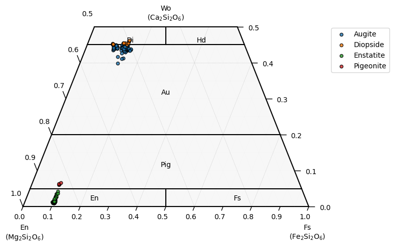
ClinopyroxeneCalculator, OrthopyroxeneCalculator, PyroxeneClassifier
``mm.ClinopyroxeneCalculator``, ``mm.OrthopyroxeneCalculator``, and ``mm.PyroxeneClassifier`` perform basic calculations associated with pyroxene-group minerals along with site allocations and additionally plots these data in a ternary diagram. mineralML adds on to the Thermobar ternary diagram by also classifying pyroxenes on the :cite:t:DHZ pyroxene ternary diagram and explicitly returning the corresponding Submineral, or the specific type of pyroxene.
mm.PyroxeneClassifier is recommended if you do not know what types of pyroxenes are present. The specific calculators can be used if the type of pyroxene is known.
[11]:
# Let's select just the pyroxenes from the training dataset
px = df_load[(df_load.Mineral=='Clinopyroxene') | (df_load.Mineral=='Orthopyroxene')]
px_class = mm.PyroxeneClassifier(px)
px_comp = px_class.calculate_components() # mm.PyroxeneClassifier wraps mm.ClinopyroxeneCalculator and mm.OrthopyroxeneCalculator into the calculation.
display(px_comp.head())
| Sample | SiO2 | TiO2 | Al2O3 | FeOt | MnO | MgO | CaO | Na2O | K2O | ... | EnFs | DiHd_2003 | Di | Fe3_Wang21 | Fe2_Wang21 | Di_h | Hd_h | Aeg_h | Jd_h | En_h | |
|---|---|---|---|---|---|---|---|---|---|---|---|---|---|---|---|---|---|---|---|---|---|
| 500 | 17MMSG37_cpx4_1 | 46.8911 | 2.8722 | 6.5948 | 8.4685 | 0.1886 | 13.8840 | 20.2569 | 0.3403 | NaN | ... | 0.181445 | 0.679835 | 0.503620 | 0.047757 | 0.218079 | 0.644230 | 0.0 | 0.0 | 0.0 | 0.166640 |
| 501 | 17MMSG37_cpx4_2 | 47.0099 | 2.8815 | 6.1648 | 8.3329 | 0.1244 | 13.3498 | 21.2249 | 0.3897 | NaN | ... | 0.139679 | 0.731564 | 0.539713 | 0.051349 | 0.210839 | 0.693298 | 0.0 | 0.0 | 0.0 | 0.122529 |
| 502 | 17MMSG37_cpx4_3 | 49.2254 | 1.9378 | 5.1564 | 7.3874 | 0.1875 | 14.5309 | 21.1051 | 0.3432 | NaN | ... | 0.148625 | 0.736030 | 0.569445 | 0.031086 | 0.198215 | 0.712806 | 0.0 | 0.0 | 0.0 | 0.139960 |
| 503 | 17MMSG37_cpx4_4 | 49.0144 | 1.8793 | 4.7032 | 7.3963 | 0.1563 | 14.5894 | 21.2841 | 0.3372 | NaN | ... | 0.142870 | 0.757924 | 0.587313 | 0.043540 | 0.187558 | 0.725445 | 0.0 | 0.0 | 0.0 | 0.129104 |
| 504 | 17MMSG37_cpx4_5 | 48.0983 | 2.4130 | 5.4135 | 7.9980 | 0.1524 | 14.0731 | 20.8235 | 0.3628 | NaN | ... | 0.154664 | 0.728051 | 0.549481 | 0.039962 | 0.210824 | 0.698229 | 0.0 | 0.0 | 0.0 | 0.142172 |
5 rows × 86 columns
[12]:
# Plot these pyroxenes!
fig, ax = px_class.plot()
/home/docs/checkouts/readthedocs.org/user_builds/mineralml/conda/stable/lib/python3.9/site-packages/ternary/plotting.py:148: UserWarning: No data for colormapping provided via 'c'. Parameters 'vmin', 'vmax' will be ignored
  ax.scatter(xs, ys, vmin=vmin, vmax=vmax, **kwargs)
EpidoteCalculator
``mm.EpidoteCalculator`` performs basic calculations and site allocations associated with epidote minerals.
[13]:
# Let's select just the epidotes from the training dataset
ep = df_load[df_load.Mineral=='Epidote']
ep_calc = mm.EpidoteCalculator(ep)
ep_comp = ep_calc.calculate_components()
display(ep_comp.head())
| Sample | SiO2 | TiO2 | Al2O3 | Fe2O3t | MnO | MgO | CaO | Na2O | K2O | ... | Al_M1M3 | Fe_M3 | Al_M3 | Fe_M1 | Al_M1 | XMn_Ep | XFe_Ep | XEp | XZo | XSum | |
|---|---|---|---|---|---|---|---|---|---|---|---|---|---|---|---|---|---|---|---|---|---|
| 600 | CL09MB009 C2 ep 20 | 37.38 | 0.01 | 21.29 | 17.060256 | 0.29 | 0.06 | 23.19 | 0.00 | 0.00 | ... | 0.999591 | 0.980426 | 4.163336e-17 | 0.042639 | 0.999591 | 0.019574 | 0.042639 | 0.937787 | 0.000000 | 1.0 |
| 601 | CL09MB009 C1 ep 19 | 37.55 | 0.03 | 22.51 | 14.970792 | 0.55 | 0.02 | 22.97 | 0.03 | 0.02 | ... | 1.112355 | 0.896992 | 6.591658e-02 | 0.000000 | 1.046439 | 0.037092 | 0.000000 | 0.896992 | 0.065917 | 1.0 |
| 602 | CL09MB010 C5 ep 26 | 37.59 | 0.02 | 21.72 | 16.148894 | 0.20 | 0.01 | 23.30 | 0.01 | 0.02 | ... | 1.037949 | 0.967450 | 1.906422e-02 | 0.000000 | 1.018885 | 0.013486 | 0.000000 | 0.967450 | 0.019064 | 1.0 |
| 603 | CL09MB010 C4 ep 25 | 36.61 | 0.00 | 19.84 | 18.049418 | 0.32 | 0.07 | 22.92 | 0.03 | 0.01 | ... | 0.902403 | 0.977949 | 0.000000e+00 | 0.127087 | 0.902403 | 0.022051 | 0.127087 | 0.850862 | 0.000000 | 1.0 |
| 604 | CL09MB010 C2 ep 24 | 39.08 | 0.02 | 23.24 | 12.925784 | 1.65 | 0.04 | 20.78 | 0.42 | 0.04 | ... | 1.166599 | 0.769399 | 1.200532e-01 | 0.000000 | 1.046546 | 0.110548 | 0.000000 | 0.769399 | 0.120053 | 1.0 |
5 rows × 67 columns
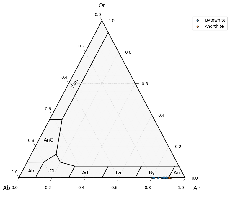
FeldsparCalculator, FeldsparClassifier
``mm.FeldsparCalculator`` and ``mm.FeldsparClassifier`` perform basic calculations associated with feldspar-group minerals along with site allocations and additionally plots these data in a ternary diagram. mineralML pulls the lines from the Thermobar ternary diagram, and further classifies data on the feldspar ternary diagram and explicitly returns the corresponding Submineral, or the specific type of feldspar.
[14]:
# Let's select just the feldspars from the training dataset
feld = df_load[(df_load.Mineral=='KFeldspar') | (df_load.Mineral=='Plagioclase')]
feld_class = mm.FeldsparClassifier(feld) # mm.FeldsparClassifier wraps mm.FeldsparCalculator into the calculation.
feld_comp = feld_class.calculate_components()
display(feld_comp.head())
| Sample | SiO2 | TiO2 | Al2O3 | FeOt | MnO | MgO | CaO | Na2O | K2O | ... | Prediction_Score | Prediction_Score_Sigma | Second_Predict_Mineral | Second_Prediction_Score | Cation_Sum | M_site | T_site | An | Ab | Or | |
|---|---|---|---|---|---|---|---|---|---|---|---|---|---|---|---|---|---|---|---|---|---|
| 1900 | K8_plag1_rtoc | 46.6657 | 0.0297 | 32.4782 | 0.5769 | 0.0013 | 0.2178 | 16.8384 | 1.7939 | 0.0031 | ... | NaN | NaN | NaN | NaN | 5.008503 | 1.004656 | 3.965077 | 0.838221 | 0.161596 | 0.000184 |
| 1901 | K8_plag1_rtoc | 44.5544 | 0.0318 | 33.0280 | 0.6945 | 0.0000 | 0.1859 | 17.5145 | 1.2080 | 0.0016 | ... | NaN | NaN | NaN | NaN | 5.012266 | 1.003164 | 3.967194 | 0.888954 | 0.110949 | 0.000097 |
| 1902 | K8_plag1_rtoc | 45.6028 | 0.0204 | 33.7199 | 0.4723 | 0.0000 | 0.1631 | 17.8024 | 1.2954 | 0.0000 | ... | NaN | NaN | NaN | NaN | 5.009193 | 1.005031 | 3.973737 | 0.883647 | 0.116353 | 0.000000 |
| 1903 | K8_plag1_rtoc | 46.0039 | 0.0134 | 33.6541 | 0.4618 | 0.0000 | 0.1837 | 17.8203 | 1.4068 | 0.0208 | ... | NaN | NaN | NaN | NaN | 5.012778 | 1.012280 | 3.969448 | 0.873940 | 0.124846 | 0.001215 |
| 1904 | K8_plag1_rtoc | 45.4534 | 0.0257 | 33.6079 | 0.4594 | 0.0151 | 0.1775 | 17.6952 | 1.3258 | 0.0080 | ... | NaN | NaN | NaN | NaN | 5.011155 | 1.006098 | 3.973252 | 0.880190 | 0.119336 | 0.000474 |
5 rows × 58 columns
[15]:
# Plot these feldspars!
fig, ax = feld_class.plot()
GarnetCalculator
``mm.GarnetCalculator`` performs basic calculations and site allocations associated with garnet minerals. This includes the Droop calculation for determining the proportion of Fe³⁺ and Fe²⁺.
[16]:
# Let's select just the garnets from the training dataset
gt = df_load[df_load.Mineral=='Garnet']
gt_calc = mm.GarnetCalculator(gt)
gt_comp = gt_calc.calculate_components()
display(gt_comp.head())
| Sample | SiO2 | TiO2 | Al2O3 | FeO | Fe2O3 | MnO | MgO | CaO | Na2O | ... | Cr_AlCr | Fe3_prop | And | Ca_corr | Alm | Prp | Sps | Grs | End_Sum | Mgno | |
|---|---|---|---|---|---|---|---|---|---|---|---|---|---|---|---|---|---|---|---|---|---|
| 700 | Lw-Ec_GR1_core | 38.52 | 0.04 | 21.84 | 27.047389 | 0.025123 | 1.49 | 5.58 | 5.82 | 0.03 | ... | 0.000000 | 0.000835 | 0.000391 | 0.483042 | 0.588929 | 0.216381 | 0.032828 | 0.161471 | 1.0 | 0.268870 |
| 701 | Lw-Ec_GR1_rim | 38.84 | 0.02 | 21.82 | 27.810000 | 0.000000 | 0.81 | 5.51 | 6.20 | 0.00 | ... | 0.000307 | 0.000000 | 0.000000 | 0.513953 | 0.599414 | 0.211697 | 0.017682 | 0.171207 | 1.0 | 0.260997 |
| 702 | Lw-Ec_GR1_reaction rim | 40.08 | 0.05 | 22.83 | 20.119372 | 0.522911 | 0.21 | 12.56 | 4.10 | 0.00 | ... | 0.000881 | 0.022852 | 0.008913 | 0.282820 | 0.427762 | 0.464563 | 0.004413 | 0.094349 | 1.0 | 0.526692 |
| 703 | Zo-Ec_MR4_core | 39.12 | 0.73 | 21.00 | 26.390000 | 0.000000 | 2.09 | 4.98 | 5.97 | 0.08 | ... | 0.002231 | 0.000000 | 0.000000 | 0.497494 | 0.586025 | 0.197126 | 0.047004 | 0.169845 | 1.0 | 0.251709 |
| 704 | Zo-Ec_MR4_rim | 39.84 | 0.06 | 22.54 | 25.270000 | 0.000000 | 0.78 | 7.74 | 4.97 | 0.03 | ... | 0.000892 | 0.000000 | 0.000000 | 0.403554 | 0.546684 | 0.298476 | 0.017090 | 0.137750 | 1.0 | 0.353160 |
5 rows × 74 columns
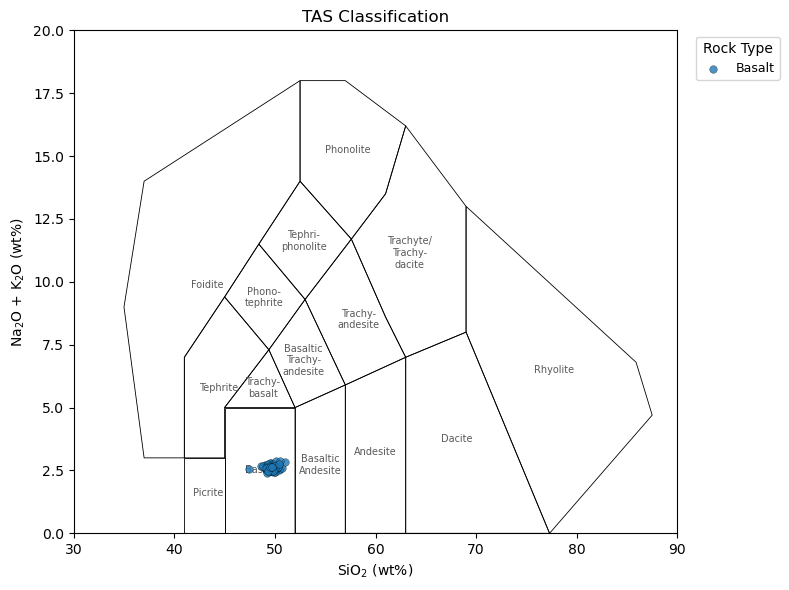
GlassCalculator, GlassClassifier
``mm.GlassCalculator`` performs basic calculations for Mg#s and ``mm.GlassClassifier`` works with these data in TAS space. mineralML pulls the lines from the pyrolite TAS diagram, and further classifies data on the TAS diagram to explicitly return the corresponding TAS classification.
[17]:
# Let's select just the glasses from the training dataset
gl = df_load[df_load.Mineral=='Glass']
gl_class = mm.GlassClassifier(gl)
gl_comp = gl_class.calculate_components()
display(gl_comp.head())
| SiO2 | TiO2 | Al2O3 | FeOt | MnO | MgO | CaO | Na2O | K2O | P2O5 | ... | K2O_mols | MgO_mols | MnO_mols | Na2O_mols | P2O5_mols | SiO2_mols | TiO2_mols | MgNo | Mineral | TAS | |
|---|---|---|---|---|---|---|---|---|---|---|---|---|---|---|---|---|---|---|---|---|---|
| 2700 | 49.96 | 1.59 | 13.73 | 11.80 | 0.21 | 7.27 | 11.88 | 2.27 | 0.25 | 0.18 | ... | 0.002654 | 0.180377 | 0.002960 | 0.036625 | 0.001268 | 0.831558 | 0.019908 | 0.523406 | Glass | Basalt |
| 2701 | 49.58 | 1.63 | 14.16 | 11.54 | 0.21 | 7.14 | 11.85 | 2.25 | 0.29 | 0.16 | ... | 0.003079 | 0.177152 | 0.002960 | 0.036303 | 0.001127 | 0.825233 | 0.020409 | 0.524463 | Glass | Basalt |
| 2702 | 49.68 | 1.65 | 14.12 | 11.98 | 0.19 | 7.30 | 11.91 | 2.27 | 0.31 | 0.17 | ... | 0.003291 | 0.181122 | 0.002678 | 0.036625 | 0.001198 | 0.826897 | 0.020660 | 0.520656 | Glass | Basalt |
| 2703 | 49.76 | 1.57 | 13.83 | 11.68 | 0.22 | 7.11 | 11.91 | 2.21 | 0.26 | 0.19 | ... | 0.002760 | 0.176408 | 0.003101 | 0.035657 | 0.001339 | 0.828229 | 0.019658 | 0.520404 | Glass | Basalt |
| 2704 | 49.17 | 1.54 | 13.73 | 11.96 | 0.22 | 7.12 | 11.88 | 2.31 | 0.25 | 0.17 | ... | 0.002654 | 0.176656 | 0.003101 | 0.037271 | 0.001198 | 0.818409 | 0.019282 | 0.514840 | Glass | Basalt |
5 rows × 28 columns
[18]:
# Plot these glasses!
fig, ax = gl_class.plot()
KalsiliteCalculator
``mm.KalsiliteCalculator`` performs basic calculations and site allocations associated with kalsilite minerals.
[19]:
# Let's select just the kalsilite from the training dataset
kal = df_load[df_load.Mineral=='Kalsilite']
kal_calc = mm.KalsiliteCalculator(gt)
kal_comp = kal_calc.calculate_components()
display(kal_comp.head())
| Sample | SiO2 | TiO2 | Al2O3 | FeOt | MnO | MgO | CaO | Na2O | K2O | ... | Predict_Mineral | Prediction_Score | Prediction_Score_Sigma | Second_Predict_Mineral | Second_Prediction_Score | Cation_Sum | A_B_site | A_site | B_site | T_site | |
|---|---|---|---|---|---|---|---|---|---|---|---|---|---|---|---|---|---|---|---|---|---|
| 700 | Lw-Ec_GR1_core | 38.52 | 0.04 | 21.84 | 27.069998 | 1.49 | 5.58 | 5.82 | 0.03 | 0.0 | ... | NaN | NaN | NaN | NaN | NaN | 2.666830 | 0.001509 | 0.0 | 0.001509 | 1.666998 |
| 701 | Lw-Ec_GR1_rim | 38.84 | 0.02 | 21.82 | 27.810000 | 0.81 | 5.51 | 6.20 | 0.00 | 0.0 | ... | NaN | NaN | NaN | NaN | NaN | 2.666179 | 0.000000 | 0.0 | 0.000000 | 1.664938 |
| 702 | Lw-Ec_GR1_reaction rim | 40.08 | 0.05 | 22.83 | 20.589953 | 0.21 | 12.56 | 4.10 | 0.00 | 0.0 | ... | NaN | NaN | NaN | NaN | NaN | 2.669927 | 0.000000 | 0.0 | 0.000000 | 1.662780 |
| 703 | Zo-Ec_MR4_core | 39.12 | 0.73 | 21.00 | 26.390000 | 2.09 | 4.98 | 5.97 | 0.08 | 0.0 | ... | NaN | NaN | NaN | NaN | NaN | 2.651971 | 0.004021 | 0.0 | 0.004021 | 1.655910 |
| 704 | Zo-Ec_MR4_rim | 39.84 | 0.06 | 22.54 | 25.270000 | 0.78 | 7.74 | 4.97 | 0.03 | 0.0 | ... | NaN | NaN | NaN | NaN | NaN | 2.657289 | 0.001469 | 0.0 | 0.001469 | 1.677539 |
5 rows × 57 columns
LeuciteCalculator
``mm.LeuciteCalculator`` performs basic calculations and site allocations associated with leucite minerals.
[20]:
# Let's select just the leucite from the training dataset
lc = df_load[df_load.Mineral=='Leucite']
lc_calc = mm.LeuciteCalculator(gt)
lc_comp = lc_calc.calculate_components()
display(lc_comp.head())
| Sample | SiO2 | TiO2 | Al2O3 | FeOt | MnO | MgO | CaO | Na2O | K2O | ... | Mineral | Source | Predict_Mineral | Prediction_Score | Prediction_Score_Sigma | Second_Predict_Mineral | Second_Prediction_Score | Cation_Sum | Channel_site | T_site | |
|---|---|---|---|---|---|---|---|---|---|---|---|---|---|---|---|---|---|---|---|---|---|
| 700 | Lw-Ec_GR1_core | 38.52 | 0.04 | 21.84 | 27.069998 | 1.49 | 5.58 | 5.82 | 0.03 | 0.0 | ... | Garnet | Usuietal2006 | NaN | NaN | NaN | NaN | NaN | 4.000245 | 0.002263 | 2.500498 |
| 701 | Lw-Ec_GR1_rim | 38.84 | 0.02 | 21.82 | 27.810000 | 0.81 | 5.51 | 6.20 | 0.00 | 0.0 | ... | Garnet | Usuietal2006 | NaN | NaN | NaN | NaN | NaN | 3.999269 | 0.000000 | 2.497406 |
| 702 | Lw-Ec_GR1_reaction rim | 40.08 | 0.05 | 22.83 | 20.589953 | 0.21 | 12.56 | 4.10 | 0.00 | 0.0 | ... | Garnet | Usuietal2006 | NaN | NaN | NaN | NaN | NaN | 4.004890 | 0.000000 | 2.494170 |
| 703 | Zo-Ec_MR4_core | 39.12 | 0.73 | 21.00 | 26.390000 | 2.09 | 4.98 | 5.97 | 0.08 | 0.0 | ... | Garnet | Usuietal2006 | NaN | NaN | NaN | NaN | NaN | 3.977956 | 0.006032 | 2.483866 |
| 704 | Zo-Ec_MR4_rim | 39.84 | 0.06 | 22.54 | 25.270000 | 0.78 | 7.74 | 4.97 | 0.03 | 0.0 | ... | Garnet | Usuietal2006 | NaN | NaN | NaN | NaN | NaN | 3.985934 | 0.002204 | 2.516309 |
5 rows × 55 columns
MeliliteCalculator
``mm.MeliliteCalculator`` performs basic calculations and site allocations associated with melilite minerals.
[21]:
# Let's select just the melilite from the training dataset
ml = df_load[df_load.Mineral=='Melilite']
ml_calc = mm.MeliliteCalculator(ml)
ml_comp = ml_calc.calculate_components()
display(ml_comp.head())
| Sample | SiO2 | TiO2 | Al2O3 | FeOt | MnO | MgO | CaO | Na2O | K2O | ... | Source | Predict_Mineral | Prediction_Score | Prediction_Score_Sigma | Second_Predict_Mineral | Second_Prediction_Score | Cation_Sum | A_site | B_site | T_site | |
|---|---|---|---|---|---|---|---|---|---|---|---|---|---|---|---|---|---|---|---|---|---|
| 1400 | S80_7 / 2 . | 41.0155 | 0.0521 | 5.6907 | 5.2198 | 0.1310 | 6.6045 | 28.6936 | 3.7814 | 0.1842 | ... | Andersenetal2012 | NaN | NaN | NaN | NaN | NaN | 4.983373 | 1.889936 | 1.038304 | 2.036016 |
| 1401 | S80_7 / 3 . | 41.5597 | 0.0501 | 5.7844 | 4.4998 | 0.0682 | 7.0200 | 30.7951 | 3.6693 | 0.1274 | ... | Andersenetal2012 | NaN | NaN | NaN | NaN | NaN | 4.993759 | 1.945095 | 1.020602 | 2.015552 |
| 1402 | S80_7 / 4 . | 41.8556 | 0.0449 | 5.9864 | 4.4798 | 0.0661 | 7.4439 | 31.3132 | 3.8040 | 0.2444 | ... | Andersenetal2012 | NaN | NaN | NaN | NaN | NaN | 5.015601 | 1.953354 | 1.045219 | 1.997863 |
| 1403 | S80_7 / 5 . | 42.2129 | 0.0428 | 6.1056 | 3.7652 | 0.0504 | 7.6324 | 33.4048 | 3.7534 | 0.0952 | ... | Andersenetal2012 | NaN | NaN | NaN | NaN | NaN | 5.024606 | 2.018621 | 1.018144 | 1.978638 |
| 1404 | S80_7 / 6 . | 41.7562 | 0.0345 | 6.3175 | 3.4506 | 0.1193 | 7.7924 | 33.8264 | 3.6398 | 0.0929 | ... | Andersenetal2012 | NaN | NaN | NaN | NaN | NaN | 5.032885 | 2.031884 | 1.029921 | 1.959559 |
5 rows × 56 columns
MuscoviteCalculator
``mm.MuscoviteCalculator`` performs basic calculations and site allocations associated with muscovite minerals.
[22]:
# Let's select just the muscovite from the training dataset
ms = df_load[df_load.Mineral=='Muscovite']
ms_calc = mm.MuscoviteCalculator(ms)
ms_comp = ms_calc.calculate_components()
display(ms_comp.head())
| Sample | SiO2 | TiO2 | Al2O3 | FeOt | MnO | MgO | CaO | Na2O | K2O | ... | Prediction_Score | Prediction_Score_Sigma | Second_Predict_Mineral | Second_Prediction_Score | Cation_Sum | X_site | Al_IV | Al_VI | M_site | T_site | |
|---|---|---|---|---|---|---|---|---|---|---|---|---|---|---|---|---|---|---|---|---|---|
| 1500 | WS5_37 | 44.80 | 0.24 | 35.12 | 0.269 | 0.04 | 3.22 | 0.16 | 0.15 | 10.57 | ... | NaN | NaN | NaN | NaN | 7.060798 | 0.934462 | 0.998085 | 1.775268 | 2.126337 | 4.0 |
| 1501 | WS5_55 | 50.08 | 0.32 | 31.65 | 0.111 | 0.00 | 3.44 | 0.01 | 0.09 | 10.43 | ... | NaN | NaN | NaN | NaN | 6.938946 | 0.880336 | 0.731883 | 1.702210 | 2.058610 | 4.0 |
| 1502 | WS5_43 | 45.68 | 0.78 | 33.05 | 0.102 | 0.00 | 3.74 | 0.00 | 0.09 | 10.09 | ... | NaN | NaN | NaN | NaN | 7.007101 | 0.879622 | 0.919963 | 1.706258 | 2.127478 | 4.0 |
| 1503 | WS2_41 | 47.72 | 0.26 | 37.70 | 0.113 | 0.00 | 1.20 | 0.00 | 0.37 | 10.32 | ... | NaN | NaN | NaN | NaN | 6.942297 | 0.891426 | 0.935662 | 1.917376 | 2.050871 | 4.0 |
| 1504 | WS2_59 | 50.45 | 0.36 | 33.83 | 0.110 | 0.01 | 2.33 | 0.00 | 0.19 | 10.82 | ... | NaN | NaN | NaN | NaN | 6.932214 | 0.906777 | 0.771740 | 1.779430 | 2.025437 | 4.0 |
5 rows × 58 columns
NephelineCalculator
``mm.NephelineCalculator`` performs basic calculations and site allocations associated with nepheline minerals.
[23]:
# Let's select just the nepheline from the training dataset
ne = df_load[df_load.Mineral=='Nepheline']
ne_calc = mm.NephelineCalculator(ne)
ne_comp = ne_calc.calculate_components()
display(ne_comp.head())
| Sample | SiO2 | TiO2 | Al2O3 | FeOt | MnO | MgO | CaO | Na2O | K2O | ... | Predict_Mineral | Prediction_Score | Prediction_Score_Sigma | Second_Predict_Mineral | Second_Prediction_Score | Cation_Sum | A_B_site | A_site | B_site | T_site | |
|---|---|---|---|---|---|---|---|---|---|---|---|---|---|---|---|---|---|---|---|---|---|
| 1600 | 10_N_1 | 42.033 | NaN | 32.705 | 0.0 | NaN | NaN | 0.105 | 15.507 | 7.859 | ... | NaN | NaN | NaN | NaN | NaN | 23.851770 | 7.916997 | 1.979838 | 5.937159 | 15.912557 |
| 1601 | 10_N_2 | 42.496 | NaN | 32.500 | 0.0 | NaN | NaN | 0.096 | 15.679 | 7.757 | ... | NaN | NaN | NaN | NaN | NaN | 23.837297 | 7.925088 | 1.946267 | 5.978821 | 15.891979 |
| 1602 | 10_N_3 | 42.074 | NaN | 32.531 | 0.0 | NaN | NaN | 0.090 | 15.625 | 7.838 | ... | NaN | NaN | NaN | NaN | NaN | 23.876813 | 7.963799 | 1.976263 | 5.987536 | 15.893955 |
| 1603 | 10_N_4 | 42.244 | NaN | 32.434 | 0.0 | NaN | NaN | 0.065 | 15.846 | 7.918 | ... | NaN | NaN | NaN | NaN | NaN | 23.927233 | 8.048425 | 1.991428 | 6.056997 | 15.865078 |
| 1604 | 10_N_5 | 42.214 | NaN | 33.003 | 0.0 | NaN | NaN | 0.100 | 15.690 | 7.884 | ... | NaN | NaN | NaN | NaN | NaN | 23.873531 | 7.940593 | 1.973025 | 5.967569 | 15.911919 |
5 rows × 57 columns
OlivineCalculator
``mm.OlivineCalculator`` performs basic calculations and site allocations associated with olivine minerals.
[24]:
# Let's select just the olivine from the training dataset
ol = df_load[df_load.Mineral=='Olivine']
ol_calc = mm.OlivineCalculator(ol)
ol_comp = ol_calc.calculate_components()
display(ol_comp.head())
| Sample | SiO2 | TiO2 | Al2O3 | FeOt | MnO | MgO | CaO | Na2O | K2O | ... | Predict_Mineral | Prediction_Score | Prediction_Score_Sigma | Second_Predict_Mineral | Second_Prediction_Score | Cation_Sum | M_site | T_site | M_site_expanded | Fo | |
|---|---|---|---|---|---|---|---|---|---|---|---|---|---|---|---|---|---|---|---|---|---|
| 1700 | CN_C_Ol1 | 39.846040 | 0.000020 | 0.019150 | 17.398750 | 0.243865 | 43.126690 | 0.219630 | 0.014950 | 0.007775 | ... | NaN | NaN | NaN | NaN | NaN | 2.997687 | 1.982656 | 1.002081 | 1.993767 | 0.815444 |
| 1701 | CN_C_Ol1' | 39.787840 | 0.010270 | 0.026165 | 17.446295 | 0.324905 | 43.227635 | 0.188190 | 0.015305 | 0.006115 | ... | NaN | NaN | NaN | NaN | NaN | 2.999612 | 1.985634 | 0.999709 | 1.997614 | 0.815385 |
| 1702 | CN_C_Ol2 | 38.896455 | 0.014615 | 0.005655 | 21.791545 | 0.349310 | 39.472920 | 0.204635 | 0.004635 | 0.006005 | ... | NaN | NaN | NaN | NaN | NaN | 2.998462 | 1.983093 | 1.000927 | 1.996348 | 0.763530 |
| 1703 | CN_C_Ol3 | 39.451170 | 0.000020 | 0.028775 | 19.528820 | 0.298085 | 41.429130 | 0.231755 | 0.000010 | 0.001825 | ... | NaN | NaN | NaN | NaN | NaN | 2.997565 | 1.982112 | 1.001395 | 1.994823 | 0.790862 |
| 1704 | CN_C_Ol3_MI2 | 39.680195 | 0.006940 | 0.019405 | 18.502340 | 0.303840 | 42.207405 | 0.226190 | 0.018970 | 0.000010 | ... | NaN | NaN | NaN | NaN | NaN | 2.997465 | 1.980623 | 1.002578 | 1.993248 | 0.802618 |
5 rows × 57 columns
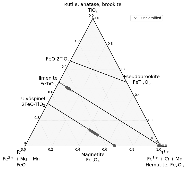
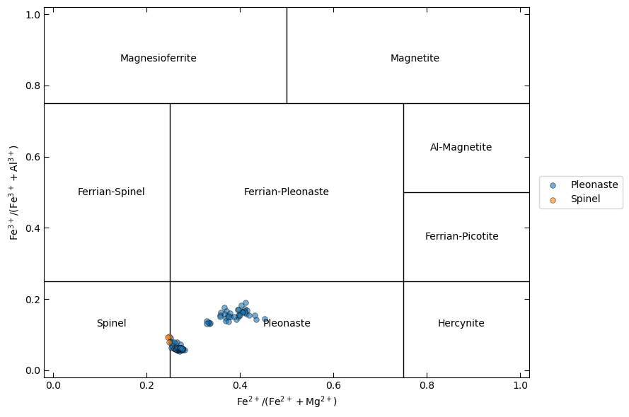
RhombohedralOxideCalculator, SpinelCalculator, OxideClassifier
``mm.RhombohedralOxideCalculator``, ``mm.SpinelCalculator``, and ``mm.OxideClassifier`` perform basic calculations associated with oxide and spinel minerals along with site allocations and additionally plots these data in a ternary diagram. This includes the Droop calculation for determining the proportion of Fe³⁺ and Fe²⁺. mineralML classifies oxides on the :cite:t:DHZ Ti⁴⁺-R³⁺-R²⁺ ternary diagram and explicitly returns the corresponding Submineral, or the specific type
of oxide, and Subspinel, if the mineral is a spinel.
mm.OxideClassifier is recommended if you do not know what types of oxides are present. The specific calculators can be used if the type of oxide is known. If there are spinels detected, the data will also be plotted on a spinel classification diagram.
[25]:
# Let's select just the oxides from the training dataset
ox = df_load[(df_load.Mineral=='Hematite') | (df_load.Mineral=='Ilmenite') | (df_load.Mineral=='Spinel') | (df_load.Mineral=='Magnetite')]
ox_class = mm.OxideClassifier(ox)
ox_comp = ox_class.calculate_components() # mm.OxideClassifier wraps mm.RhombohedralOxideCalculator and mm.SpinelCalculator into the calculation.
display(ox_comp.head())
| Sample Name | SiO2 | TiO2 | Al2O3 | FeOt | MnO | MgO | CaO | Na2O | K2O | ... | Fe2t_cat_4ox | Fe2_cat_4ox | Fe3_cat_4ox | Mn_cat_4ox | Mg_cat_4ox | Ca_cat_4ox | Na_cat_4ox | K_cat_4ox | P_cat_4ox | Cr_cat_4ox | |
|---|---|---|---|---|---|---|---|---|---|---|---|---|---|---|---|---|---|---|---|---|---|
| 800 | NaN | 0.396 | 0.026 | 0.218 | 86.979284 | NaN | 0.016 | 0.096 | NaN | 0.003 | ... | NaN | NaN | NaN | NaN | NaN | NaN | NaN | NaN | NaN | NaN |
| 801 | NaN | 0.519 | 0.063 | 0.415 | 87.037278 | NaN | NaN | 0.084 | 0.041 | 0.011 | ... | NaN | NaN | NaN | NaN | NaN | NaN | NaN | NaN | NaN | NaN |
| 802 | NaN | 0.395 | 0.071 | 0.757 | 86.374344 | 0.031 | 0.013 | 0.109 | NaN | 0.002 | ... | NaN | NaN | NaN | NaN | NaN | NaN | NaN | NaN | NaN | NaN |
| 803 | NaN | 0.378 | 0.151 | 0.350 | 86.856296 | NaN | 0.010 | 0.102 | NaN | 0.007 | ... | NaN | NaN | NaN | NaN | NaN | NaN | NaN | NaN | NaN | NaN |
| 804 | NaN | 0.420 | 0.028 | 0.324 | 87.157266 | NaN | 0.011 | 0.131 | NaN | 0.004 | ... | NaN | NaN | NaN | NaN | NaN | NaN | NaN | NaN | NaN | NaN |
5 rows × 92 columns
[26]:
# Plot these oxides!
fig, ax = ox_class.plot()
/home/docs/checkouts/readthedocs.org/user_builds/mineralml/conda/stable/lib/python3.9/site-packages/ternary/plotting.py:148: UserWarning: No data for colormapping provided via 'c'. Parameters 'vmin', 'vmax' will be ignored
  ax.scatter(xs, ys, vmin=vmin, vmax=vmax, **kwargs)
QuartzCalculator
``mm.QuartzCalculator`` performs basic calculations and site allocations associated with quartz minerals.
[27]:
# Let's select just the quartz from the training dataset
qz = df_load[df_load.Mineral=='SiO2_Polymorph']
qz_calc = mm.QuartzCalculator(qz)
qz_comp = qz_calc.calculate_components()
display(qz_comp.head())
| Sample | SiO2 | TiO2 | Al2O3 | FeOt | MnO | MgO | CaO | Na2O | K2O | ... | Cr_cat_2ox | Mineral | Source | Predict_Mineral | Prediction_Score | Prediction_Score_Sigma | Second_Predict_Mineral | Second_Prediction_Score | Cation_Sum | T_site | |
|---|---|---|---|---|---|---|---|---|---|---|---|---|---|---|---|---|---|---|---|---|---|
| 2000 | OM08-206A_2 | 99.70 | 0.00 | 0.00 | 0.30 | 0.03 | 0.0 | 0.00 | 0.01 | 0.02 | ... | 0.0 | SiO2_Polymorph | Streitetal2012 | NaN | NaN | NaN | NaN | NaN | 1.001721 | 0.998504 |
| 2001 | Gon05230ph-j | 96.89 | 0.00 | 0.01 | 0.01 | 0.00 | 0.0 | 0.03 | 0.03 | 0.01 | ... | 0.0 | SiO2_Polymorph | Kleinsasseretal2008 | NaN | NaN | NaN | NaN | NaN | 1.000788 | 0.999639 |
| 2002 | Gon05262a1-6 | 97.61 | 0.00 | 0.02 | 0.06 | 0.00 | 0.0 | 0.01 | 0.05 | 0.02 | ... | 0.0 | SiO2_Polymorph | Kleinsasseretal2008 | NaN | NaN | NaN | NaN | NaN | 1.001312 | 0.999435 |
| 2003 | Gon05262A1ph-i | 96.59 | 0.00 | 0.02 | 0.00 | 0.01 | 0.0 | 0.01 | 0.03 | 0.01 | ... | 0.0 | SiO2_Polymorph | Kleinsasseretal2008 | NaN | NaN | NaN | NaN | NaN | 1.000711 | 0.999778 |
| 2004 | Gon05262a2ph-b | 96.99 | 0.02 | 0.02 | 0.00 | 0.00 | 0.0 | 0.01 | 0.03 | 0.00 | ... | 0.0 | SiO2_Polymorph | Kleinsasseretal2008 | NaN | NaN | NaN | NaN | NaN | 1.000565 | 0.999856 |
5 rows × 54 columns
RutileCalculator
``mm.RutileCalculator`` performs basic calculations and site allocations associated with rutile minerals.
[28]:
# Let's select just the rutile from the training dataset
rt = df_load[df_load.Mineral=='Rutile']
rt_calc = mm.RutileCalculator(rt)
rt_comp = rt_calc.calculate_components()
display(rt_comp.head())
| Sample | SiO2 | TiO2 | Al2O3 | FeOt | MnO | MgO | CaO | Na2O | K2O | ... | Cr_cat_2ox | Mineral | Source | Predict_Mineral | Prediction_Score | Prediction_Score_Sigma | Second_Predict_Mineral | Second_Prediction_Score | Cation_Sum | M_site | |
|---|---|---|---|---|---|---|---|---|---|---|---|---|---|---|---|---|---|---|---|---|---|
| 2100 | E2718C_1_ | 0.0091 | 98.4337 | 0.0236 | 0.2144 | 0.0089 | NaN | NaN | NaN | NaN | ... | 0.002103 | Rutile | Penniston-Dorlandetal2018 | NaN | NaN | NaN | NaN | NaN | 1.001877 | 0.996762 |
| 2101 | E2718C_2_ | 0.0075 | 98.6836 | 0.0379 | 0.2062 | 0.0033 | NaN | NaN | NaN | NaN | ... | 0.002132 | Rutile | Penniston-Dorlandetal2018 | NaN | NaN | NaN | NaN | NaN | 1.001859 | 0.996674 |
| 2102 | E2718C_3_ | 0.0178 | 98.4385 | 0.0374 | 0.2277 | 0.0152 | NaN | NaN | NaN | NaN | ... | 0.002044 | Rutile | Penniston-Dorlandetal2018 | NaN | NaN | NaN | NaN | NaN | 1.002027 | 0.996415 |
| 2103 | E2718C_4_ | 0.0051 | 98.5087 | 0.0394 | 0.2048 | 0.0000 | NaN | NaN | NaN | NaN | ... | 0.002188 | Rutile | Penniston-Dorlandetal2018 | NaN | NaN | NaN | NaN | NaN | 1.001855 | 0.996670 |
| 2104 | E2718C_5_ | 0.0153 | 98.5736 | 0.0429 | 0.1740 | 0.0000 | NaN | NaN | NaN | NaN | ... | 0.002386 | Rutile | Penniston-Dorlandetal2018 | NaN | NaN | NaN | NaN | NaN | 1.001744 | 0.996517 |
5 rows × 54 columns
SerpentineCalculator
``mm.SerpentineCalculator`` performs basic calculations and site allocations associated with serpentine minerals.
[29]:
# Let's select just the serpentine from the training dataset
srp = df_load[df_load.Mineral=='Serpentine']
srp_calc = mm.SerpentineCalculator(srp)
srp_comp = srp_calc.calculate_components()
display(srp_comp.head())
| Sample | SiO2 | TiO2 | Al2O3 | FeOt | MnO | MgO | CaO | Na2O | K2O | ... | Predict_Mineral | Prediction_Score | Prediction_Score_Sigma | Second_Predict_Mineral | Second_Prediction_Score | Cation_Sum | M_site | T_site | Mgno | Feno | |
|---|---|---|---|---|---|---|---|---|---|---|---|---|---|---|---|---|---|---|---|---|---|
| 2200 | OM15-6 | 41.25742 | NaN | 1.34979 | 4.38996 | NaN | 39.54539 | NaN | NaN | NaN | ... | NaN | NaN | NaN | NaN | NaN | 10.007675 | 5.930137 | 4.057754 | 0.941374 | 0.058626 |
| 2201 | OM15-6 | 45.03778 | 0.03470 | 0.61300 | 4.27731 | 0.04921 | 38.90302 | NaN | NaN | NaN | ... | NaN | NaN | NaN | NaN | NaN | 9.838212 | 5.639891 | 4.188997 | 0.941903 | 0.058097 |
| 2202 | OM15-6 | 44.78683 | NaN | 0.07731 | 5.53723 | NaN | 36.07066 | NaN | NaN | NaN | ... | NaN | NaN | NaN | NaN | NaN | 9.762243 | 5.520180 | 4.242063 | 0.920709 | 0.079291 |
| 2203 | OM15-6 | 39.87580 | NaN | NaN | 8.69485 | 0.05758 | 36.68905 | NaN | NaN | NaN | ... | NaN | NaN | NaN | NaN | NaN | 10.061990 | 6.123979 | 3.938010 | 0.882652 | 0.117348 |
| 2204 | OM15-6 | 41.42825 | 0.02485 | 0.70973 | 4.95897 | 0.12620 | 37.89634 | 0.38051 | NaN | NaN | ... | NaN | NaN | NaN | NaN | NaN | 9.966206 | 5.852836 | 4.072289 | 0.931610 | 0.068390 |
5 rows × 57 columns
TitaniteCalculator
``mm.TitaniteCalculator`` performs basic calculations and site allocations associated with titanite minerals.
[30]:
# Let's select just the titanite from the training dataset
tit = df_load[df_load.Mineral=='Titanite']
tit_calc = mm.TitaniteCalculator(tit)
tit_comp = tit_calc.calculate_components()
display(tit_comp.head())
| Sample | SiO2 | TiO2 | Al2O3 | Fe2O3t | MnO | MgO | CaO | Na2O | K2O | ... | Prediction_Score | Prediction_Score_Sigma | Second_Predict_Mineral | Second_Prediction_Score | Cation_Sum | VII_site | M_site | T_site | Al_IV | Al_VI | |
|---|---|---|---|---|---|---|---|---|---|---|---|---|---|---|---|---|---|---|---|---|---|
| 2400 | REG-19_titanite_1 | 29.3211 | 33.0262 | 1.3941 | 3.228223 | 0.0339 | 0.0760 | 26.5311 | 0.1435 | 0.0327 | ... | NaN | NaN | NaN | NaN | 3.042775 | 1.007854 | 1.009891 | 1.024027 | -0.024027 | 0.081407 |
| 2401 | REG-19_titanite_2 | 29.4279 | 32.8271 | 1.4883 | 3.040504 | 0.0106 | 0.0771 | 26.3000 | 0.1441 | 0.0234 | ... | NaN | NaN | NaN | NaN | 3.039107 | 1.001705 | 1.006433 | 1.030654 | -0.030654 | 0.092083 |
| 2402 | REG-26_titanite_3 | 28.3689 | 34.0591 | 0.9669 | 2.756982 | 0.0000 | 0.0450 | 25.3917 | 0.0875 | 0.0219 | ... | NaN | NaN | NaN | NaN | 3.020337 | 0.979827 | 1.028573 | 1.011937 | -0.011937 | 0.052583 |
| 2403 | REG-26_titanite_4 | 28.4892 | 34.1129 | 0.9527 | 2.763650 | 0.0425 | 0.0504 | 25.3284 | 0.1785 | 0.0219 | ... | NaN | NaN | NaN | NaN | 3.023153 | 0.981408 | 1.026900 | 1.013564 | -0.013564 | 0.053508 |
| 2404 | REG-26_titanite_5 | 28.6437 | 34.3889 | 0.9107 | 2.492465 | 0.0436 | 0.0599 | 25.7252 | 0.1730 | 0.0394 | ... | NaN | NaN | NaN | NaN | 3.026083 | 0.991876 | 1.019535 | 1.013364 | -0.013364 | 0.051335 |
5 rows × 58 columns
TourmalineCalculator
``mm.TourmalineCalculator`` performs basic calculations and site allocations associated with tourmaline minerals.
[31]:
# Let's select just the tourmaline from the training dataset
trm = df_load[df_load.Mineral=='Tourmaline']
trm_calc = mm.TourmalineCalculator(trm)
trm_comp = trm_calc.calculate_components()
display(trm_comp.head())
| Sample | SiO2 | TiO2 | Al2O3 | FeOt | MnO | MgO | CaO | Na2O | K2O | ... | Predict_Mineral | Prediction_Score | Prediction_Score_Sigma | Second_Predict_Mineral | Second_Prediction_Score | Cation_Sum | X_site | Y_site | Z_site | T_site | |
|---|---|---|---|---|---|---|---|---|---|---|---|---|---|---|---|---|---|---|---|---|---|
| 2500 | Tourmaline1 | 36.47 | 0.82 | 30.79 | 4.13 | NaN | 9.52 | 0.74 | 2.36 | NaN | ... | NaN | NaN | NaN | NaN | NaN | 20.009383 | 1.114422 | 11.195858 | 11.195858 | 7.571047 |
| 2501 | Tourmaline2 | 35.37 | 1.23 | 30.34 | 5.00 | NaN | 9.01 | 1.24 | 2.26 | NaN | ... | NaN | NaN | NaN | NaN | NaN | 20.064564 | 1.200477 | 11.220063 | 11.233360 | 7.436196 |
| 2502 | Tourmaline3 | 36.89 | 0.86 | 31.06 | 4.07 | NaN | 9.49 | 0.57 | 2.57 | NaN | ... | NaN | NaN | NaN | NaN | NaN | 20.021356 | 1.150535 | 11.139630 | 11.149387 | 7.588356 |
| 2503 | Tourmaline4 | 36.80 | 0.69 | 31.12 | 3.64 | NaN | 9.75 | 0.49 | 2.62 | NaN | ... | NaN | NaN | NaN | NaN | NaN | 20.044231 | 1.155443 | 11.185088 | 11.194868 | 7.586908 |
| 2504 | Tourmaline5 | 36.80 | 0.79 | 30.91 | 3.99 | NaN | 9.55 | 0.69 | 2.44 | NaN | ... | NaN | NaN | NaN | NaN | NaN | 20.004314 | 1.129609 | 11.152047 | 11.152047 | 7.599927 |
5 rows × 57 columns
ZirconCalculator
``mm.ZirconCalculator`` performs basic calculations and site allocations associated with zircon minerals.
[32]:
# Let's select just the zircon from the training dataset
zr = df_load[df_load.Mineral=='Zircon']
zr_calc = mm.ZirconCalculator(zr)
zr_comp = zr_calc.calculate_components()
display(zr_comp.head())
| Sample | SiO2 | TiO2 | Al2O3 | FeOt | MnO | MgO | CaO | Na2O | K2O | ... | Mineral | Source | Predict_Mineral | Prediction_Score | Prediction_Score_Sigma | Second_Predict_Mineral | Second_Prediction_Score | Cation_Sum | M_site | T_site | |
|---|---|---|---|---|---|---|---|---|---|---|---|---|---|---|---|---|---|---|---|---|---|
| 2600 | Zrn-I | 32.816 | 0.005 | 0.000 | 0.007 | NaN | NaN | 0.000 | 0.008 | NaN | ... | Zircon | Wangetal2023 | NaN | NaN | NaN | NaN | NaN | 2.000274 | 0.982324 | 1.016463 |
| 2601 | HA5_#1 | 31.153 | 0.128 | 0.054 | 0.380 | 0.073 | 0.020 | 0.016 | 0.023 | 0.013 | ... | Zircon | Abuamarahetal2022 | NaN | NaN | NaN | NaN | NaN | 2.007996 | 0.990713 | 0.993523 |
| 2602 | HA6_#2 | 31.358 | 0.123 | 0.027 | 0.372 | 0.146 | 0.027 | 0.023 | 0.039 | 0.003 | ... | Zircon | Abuamarahetal2022 | NaN | NaN | NaN | NaN | NaN | 2.009342 | 0.988635 | 0.995448 |
| 2603 | HA7_#3 | 31.213 | 0.114 | 0.032 | 0.210 | 0.113 | 0.033 | 0.028 | 0.034 | 0.007 | ... | Zircon | Abuamarahetal2022 | NaN | NaN | NaN | NaN | NaN | 2.007003 | 0.992636 | 0.994217 |
| 2604 | HA8_#4 | 31.318 | 0.020 | 0.016 | 0.073 | 0.025 | 0.026 | 0.018 | 0.044 | 0.002 | ... | Zircon | Abuamarahetal2022 | NaN | NaN | NaN | NaN | NaN | 2.003417 | 0.989548 | 1.001162 |
5 rows × 59 columns